Inverse Analysis of Strata in Seepage Field Based on Regularization Method and Geostatistics Theory

Abstract

During the construction of underground engineering, the prediction of groundwater distribution and rock body permeability is essential for evaluating the safety of the project and guiding subsequent design and construction. This article proposes an objective function that solves an underdetermined inverse analysis problem based on the least-squares theory and regularization method and uses geostatistics theory and the variogram function to describe the spatial characteristics of the actual engineering system. It also establishes an optimization model of the analysis stratum seepage field and puts forward the method of using on-site test observation data to solve the stratum penetration coefficient. Relying on the foundation pit project of the Lingshanwei Station of Qingdao Metro, the on-site pumping and packer permeability test was conducted for different strata venues in the foundation pit, and the on-site water-head observation value was obtained. Physical detection of the influence area of foundation pit excavation confirms the correctness of the model from the region and verifies the accuracy of the model on the value through the on-site pumping test. Results show that the accuracy of the use of this objective function to solve the underdetermined inverse problem is above 85%, which proves the effectiveness of the method. The stratigraphic geological information obtained by the inverse analysis model provides an important basis for engineering design and security construction.

1. Introduction

In the process of underground engineering construction, it is very important to determine the permeability of rock and soil mass and the distribution of groundwater [1,2]. In the early stage of project construction, it is often necessary to carry out numerous geological investigations on the rock and soil mass in the project construction area. Drilling tests are a common survey method for engineering geology and hydrogeological data. By arranging drilling at the project site and conducting on-site water pressure or pumping tests, the permeability coefficient of the stratum near the drilling can be calculated. However, geological conditions, testing construction, testing equipment, the environment, and other factors can all affect the test. It is difficult to obtain comprehensive hydrogeological information only through limited drilling data, and the obtained observation data usually have some errors. Therefore, this paper uses the on-site drilling test data to solve the permeability coefficient by establishing the solution model of the inverse problem.

In terms of the inverse analysis of seepage fields, Li [3] carried out an inverse analysis of the permeability coefficient of a tailings dam based on actual engineering geology and hydrogeological drilling data but only established a finite element model for the inversion analysis of the permeability coefficient based on actual drilling data without studying inversion theory. Zhang [4] used Midas GTS NX 2018 software to calculate the permeability coefficient based on on-site pumping test data but did not consider conducting back analysis on the formation seepage field. P. K. Kitanidis [5] proposed an implementation method for free matrices using the Gauss–Newton method of Jacobian matrices, which improves the scalability of geological statistical inversion problems. However, only theoretical analysis was conducted on the inversion problem, and no research was conducted on the practical engineering application. A. Bárdossy [6] proposed a new Gaussian and non-Gaussian inversion method for groundwater flow. Yang [7] used Modflow-2005 numerical simulation software to carry out inverse analysis on pumping test data. P. K. Kitanidis [8,9] proposed the quasi-linear theory of geostatistical solutions for inverse problems, extending the geostatistical method to a method for solving inverse problems involving spatial distribution parameters and process equations. Zhang [10] studied the influence of temperature data on the characterization of reservoir permeability by calculating the joint inversion of flow and temperature observations. Capriotti [11] used fluid flow in porous media and combined it with delayed gravity response to invert permeability distribution. Guan [12] studied the permeability of seismic logging in fluid-saturated porous formations through inversion. The load and strain rate-related characteristics of rocks and cemented soils are of great significance for determining their engineering properties. Maqsood [13] conducted unconfined monotonic tests at different strain rates to study the effects of creep and cyclic loading on the mechanical properties of boundary geotechnical materials (i.e., Gypsum Mixed Sand (GMS)) produced in the laboratory. Ojala [14] studied the effect of loading rate on the permeability of porous sandstone by conducting triaxial compression tests at different strain rates and temperatures. It was found that the evolution of permeability depends on the applied loading rate, and the decrease in initial permeability increases with the decrease in loading rate. This means that large initial compaction can be achieved under low strain rate testing. Savvides A. A. [15,16] used Monte Carlo simulation methods to test and evaluate the critical state-line inclination angle of soil and the permeability of the continuum and obtained that the failure load and displacement of nonlinear behavior soil follow a Gaussian normal distribution. Matthies H G [17] studied the main sources of uncertainty involved in structural and solid analysis and proposed methods for handling them, using stochastic modeling to solve mathematical model problems. Sett K [18] proposed an evolutionary solution for the probability density function (PDF) of the elastic–plastic, stress–strain relationship in a material model with parameter uncertainty. Li [19] established a spatially variable undrained shear-strength model using non-stationary random fields and studied the effect of spatial undrained shear strength on the performance of strip foundations. Deidda [20] studied a regularization algorithm for inverting nonlinear mathematical models in applied geophysics. Lee [21] used a global optimization algorithm to solve the problem of the optimal solution of nonlinear functions. Wang [22] built a full-range weighting method for the hydrogeological parameter inversion of a multi-observation logging pumping test and realized the optimization solution of objective function based on a hybrid particle swarm optimization algorithm. R. L. Cooley [23,24] proposed two types of prior information: prior information with known reliability (i.e., bias and random error structures) and prior information composed of the best available estimate of unknown reliability, and studied the factors that affect the accuracy of parameter estimation in nonlinear regression groundwater flow models. Lv [25] introduced a global optimization algorithm in the inverse analysis of geotechnical engineering to solve the minimum of the objective function. Many scholars have studied the calculation method of the permeability coefficient [26,27,28]. The above inverse analysis is based on parameters such as flow, water head, water storage coefficient, water inflow, and water-stop curtain boundary, and these parameters themselves have certain uncertainties. In addition, they are greatly affected by environmental conditions and other objective factors. Therefore, it is difficult to accurately obtain stratum permeability by using these parameters. The above optimization methods are mainly used to solve complex nonlinear multimodal functions, while there is less research on nonlinear underdetermined problems.

Aiming at the shortcomings of the above research, based on the least-squares theory and regularization method, an objective function of an underdetermined inverse analysis problem is proposed, and geostatistical theory and variation function are used to describe the spatial characteristics of practical engineering systems. Based on the foundation pit project of Qingdao Lingshanwei Station, on-site tests were carried out, and the permeability coefficient inverse analysis was calculated using the drilling test data. The distribution of the permeability coefficient of each stratum in the excavation area of the foundation pit was obtained. The hydrogeological information obtained from the inverse analysis model provides an important basis for engineering design and safe construction.

2. Establishment of Inverse Analysis Model

2.1. Inverse Problem Theory

In practical engineering systems, there is often a partial differential equation containing unknown coefficients or parameters, and its unknown parameters change with the spatial position. In the process of its forward solution, the forward model of geophysical problems can be expressed as:

Y = F s

(1)

where s is the set of unknown parameters in space, Y is the expected measurement values of the forward model, and F is the forward mapping between unknown parameters and expected measurement values.

Generally, F can be either linear or nonlinear. However, most geophysical problems are nonlinear. Some inverse problems in geophysical problems can be effectively approximated as linear problems, including some imaging problems in seismic and ground-penetrating radar applications [29,30]. Therefore, F is assumed to be a system of linear equations.

Considering the measurement error of the on-site test data, in order not to lose generality, there are:

$$\mathit{y}=\mathit{F}\mathit{s}+\mathsf{\Delta }\mathit{b}$$

(2)

where y is a set of measurement values, and Δb is the error between the measurement values and the expected measurement values.

Because the measurement data contain errors, and the matrix F is often not square or irreversible, it is difficult to solve unknown parameters. For such problems, the common method is to minimize the errors as much as possible, which is more conducive to error-free solutions. Among them, the most common method is to take the minimum of the error square sum as the approximate value—that is, the least-squares method:

$$\arg {\min }_{\mathit{s}}{‖\mathit{y}-\mathit{F}\mathit{s}‖}_2^2$$

(3)

Assuming that the error Δb follows a Gaussian distribution with mean 0 and variance σ² (also known as a normal distribution), then, when both F and s are determined, y follows a Gaussian distribution with a mean value of Fs and a variance of σ², and this satisfies the Gaussian distribution law [30]:

$$\mathit{p}(\mathit{y})=\frac{1}{\sqrt{2}\mathit{\sigma }}\exp \left[\frac{-{(\mathit{y}-\mathit{F}\mathit{s})}^2}{2{\mathit{\sigma }}^2}\right]$$

(4)

For m independent observation data, the joint distribution satisfies:

$$\mathit{p}(\mathit{y})=\frac{\mathit{m}}{\sqrt{2}\mathit{\sigma }}\exp \left[-\frac{{\mathit{\sigma }}^{-2}}{2}{\displaystyle \sum _{\mathit{i}=1}^{\mathit{m}}{({\mathit{y}}_{\mathit{i}}-\mathit{F}\mathit{s})}^2}\right]$$

(5)

To maximize the probability of the random variable y, there must be:

$$\mathit{E}={\displaystyle \sum _{\mathit{i}=1}^{\mathit{m}}{({\mathit{y}}_{\mathit{i}}-\mathit{F}\mathit{s})}^2}=\min$$

(6)

Formula (6) is the definition of the least-squares method without constraints, which is equivalent to Formula (3).

For a normal distribution with two random variables (s₁, s₂), the joint probability density function can be written as:

$$\mathit{p}({\mathit{s}}_{\mathbf{1}},{\mathit{s}}_{\mathbf{2}})=\frac{1}{2\mathit{\pi }{({\mathit{\sigma }}_1^2{\mathit{\sigma }}_2^2-{\mathit{\sigma }}_{12}^2)}^{1/2}}\exp \left\{-\frac{{\mathit{\sigma }}_1^2{\mathit{\sigma }}_2^2}{2({\mathit{\sigma }}_1^2{\mathit{\sigma }}_2^2-{\mathit{\sigma }}_{12}^2)}\cdot \left[{\left(\frac{{\mathit{s}}_1-{\mathit{a}}_1}{{\mathit{\sigma }}_1}\right)}^2-2\frac{{\mathit{\sigma }}_{12}}{{\mathit{\sigma }}_1{\mathit{\sigma }}_2}\cdot \frac{{\mathit{s}}_1-{\mathit{a}}_1}{{\mathit{\sigma }}_1}\cdot \frac{{\mathit{s}}_2-{\mathit{a}}_2}{{\mathit{\sigma }}_2}+{\left(\frac{{\mathit{s}}_2-{\mathit{a}}_2}{{\mathit{\sigma }}_2}\right)}^2\right]\right\}$$

(7)

Let $\mathit{\xi }=\frac{{\mathit{\sigma }}_{12}}{{\mathit{\sigma }}_{\mathbf{1}}{\mathit{\sigma }}_{\mathbf{2}}}$, the above formula be written as:

$$\mathit{p}({\mathit{s}}_1,{\mathit{s}}_2)=\frac{1}{2\mathit{\pi }{\mathit{\sigma }}_1{\mathit{\sigma }}_2\sqrt{1-{\mathit{\xi }}^2}}\exp \left\{-\frac{1}{2(1-{\mathit{\xi }}^2)}\cdot \left[{\left(\frac{{\mathit{s}}_1-{\mathit{a}}_1}{{\mathit{\sigma }}_1}\right)}^2-2\mathit{\xi }\cdot \frac{{\mathit{s}}_1-{\mathit{a}}_1}{{\mathit{\sigma }}_1}\cdot \frac{{\mathit{s}}_2-{\mathit{a}}_2}{{\mathit{\sigma }}_2}+{\left(\frac{{\mathit{s}}_2-{\mathit{a}}_2}{{\mathit{\sigma }}_2}\right)}^2\right]\right\}$$

(8)

Represented in matrix form, there are:

$$\mathit{s}=\left[\begin{array}{l}{\mathit{s}}_1\\ {\mathit{s}}_2\end{array}\right],\mathit{a}=\left[\begin{array}{l}{\mathit{a}}_1\\ {\mathit{a}}_2\end{array}\right],\mathit{Z}=\left[\begin{array}{cc}{\mathit{\sigma }}_1^2& {\mathit{\sigma }}_{12}\\ {\mathit{\sigma }}_{12}& {\mathit{\sigma }}_2^2\end{array}\right]$$

(9)

The probability density formula can be further written as:

$$\mathit{p}({\mathit{s}}_1,{\mathit{s}}_2)=\frac{1}{2\mathit{\pi }{\left|\mathit{Z}\right|}^{1/2}}\exp \left\{-\frac{1}{2}{(\mathit{s}-\mathit{a})}^{\mathit{T}}{\mathit{Z}}^{-1}(\mathit{s}-\mathit{a})\right\}$$

(10)

where a₁ is the mean of s₁, a₂ is the mean of s₂, σ₁ is the standard deviation of s₁, σ₂ is the standard deviation of s₂, ξ is the correlation coefficient, and Z is the covariance matrix.

By extending it to n-dimensional form, we can obtain that the solution of ${‖\mathit{y}-\mathit{F}\mathit{s}‖}_2^2$ is equivalent to the maximum likelihood estimation under the assumption of a Gaussian distribution when the average measurement error is zero [31,32,33].

$$\mathit{p}(\mathit{y})=\mathit{K}\cdot \exp \left\{-\frac{1}{2}{(\mathit{y}-\mathit{F}\mathit{s})}^{\mathit{T}}{\mathbf{R}}^{-1}(\mathit{y}-\mathit{F}\mathit{s})\right\}$$

(11)

where K is a constant related to the Gaussian distribution, and R is the covariance matrix.

According to the principle of least squares, in the absence of regularization constraints, the objective function [31,32] can be written as:

$$\mathit{L}(\mathit{s})={‖\mathit{y}-\mathit{F}\mathit{s}‖}_2^2$$

(12)

The objective function [31,32] corresponding to the L₂ regularization constraint can be written as:

$$\mathit{L}(\mathit{s})={‖\mathit{y}-\mathit{F}\mathit{s}‖}_2^2+\mathit{\lambda }{‖\mathit{s}‖}_2^2$$

(13)

where ${‖\mathit{y}-\mathit{F}\mathit{s}‖}_2^2$ is the Euclidean norm, ${‖\mathit{s}‖}_2^2$ is the L₂ regularization term, and λ is the regularization parameter.

Take the logarithm of Formula (11) and remove the irrelevant constant term to obtain:

$$\mathit{L}(\mathit{s})={(\mathit{y}-\mathit{F}\mathit{s})}^{\mathit{T}}{\mathbf{R}}^{-1}(\mathit{y}-\mathit{F}\mathit{s})$$

(14)

Therefore, the L₂ norm means that the measurement data error follows the statistical law of Gaussian normal distribution.

2.2. Establishment of Objective Function

For the seepage field in a specific area of the underground project, it is necessary to find a set of partial differential equations that can well describe the spatial location change of the permeability coefficient. In the process of establishing its mathematical model, because the coefficients, boundary conditions, source-sink terms, etc. of the partial differential equations are mostly difficult to obtain, the permeability coefficient is inversely calculated through a series of measurement results using the inverse analysis method. Specifically, if the number of unknown parameters n is greater than the number of measurement data m, it will be an underdetermined problem. Based on the linear algebra theory, there will be an infinite number of solutions that meet the equations, and the error is 0. In other words, the solution is not unique, and there will be an infinite number of solutions that meet the measurement values. The reason is that although the measurement values provide some information to determine the model parameters, it is not enough to determine all the parameters. This kind of problem belongs to an underdetermined inverse problem, and the model in this paper belongs to this kind of problem.

To find the solution to the underdetermined inverse problem, it is necessary to find an optimal solution from an infinite number of solutions, and data fitting alone is not enough to obtain the optimal solution. Therefore, when solving Equation (1), some information not included in the observation data must be added, which is usually called “prior information”, and its main purpose is to supplement the information missing in determining model parameters [29]. In underground engineering, the geological changes are extremely complex, and it is difficult to accurately predict the geological structure of spatial changes. In most cases, the average value is used to describe a certain variable. For example, in describing the permeability, porosity, and rock fluctuation in space, the average function is often used to express the structural characteristics—that is, the average value is used as the target to obtain a solution with zero error to express the structural characteristics, instead of taking the minimum value as the objective to obtain a solution with zero error. Therefore, this article adopts an average function (i.e., average value) and represents the structural characteristics of the seepage field through a variation function.

s represents the variables that need to be estimated in the space, and the mean parameter is used to β express:

$$\mathit{E}[\mathit{s}]=\mathbf{X}\beta$$

(15)

where E [] is the expected value, X is the n-dimensional row vector whose elements are all equal 1, and β is the average value of unknown parameters in the seepage field.

In addition, s has a covariance matrix that can be represented as:

$$\mathbf{G}=\mathit{E}[(\mathit{s}-\mathbf{X}\mathit{\beta }){(\mathit{s}-\mathbf{X}\mathit{\beta })}^{\mathit{T}}]$$

(16)

According to theoretical analysis, there are:

$$\mathit{E}={\displaystyle \sum _{\mathit{i}=1}^{\mathit{m}}{(\mathit{s}-\mathbf{X}\beta )}^2}=\min$$

(17)

In this paper, the objective function of the geophysical inverse problem is constructed based on the least-squares theory and L₂ regularization. The objective function can be expressed by the sum of the fitness term and regularization term:

$$\mathit{L}={(\mathit{y}-\mathit{F}\mathit{s})}^{\mathrm{T}}{\mathbf{R}}^{-1}(\mathit{y}-\mathit{F}\mathit{s})+\mathit{\lambda }{(\mathit{s}-\mathbf{X}\beta )}^{\mathrm{T}}{\mathbf{G}}^{-1}(\mathit{s}-\mathbf{X}\beta )$$

(18)

where y is the m-dimensional row vector of a group of measurement values, s is the n-dimensional row vector of unknown parameter values, R is the m-by-m covariance matrix of measurement errors, λ is the regularization parameter, and G is the spatial covariance matrix.

Since the on-site tests were carried out on the measure points at different locations, it can be considered that the measurement data error is independent of the variance σ_R² distribution is consistent, i.e.,

$$\mathbf{R}={\mathit{\sigma }}_{\mathit{R}}^2\mathbf{I}$$

(19)

where I is the identity matrix of m × m.

Usually, variables with spatial correlation have two main parts of variation: one is the randomness of spatial distribution influenced by many local and complex uncertainty factors; the second is the continuity of spatial distribution in the macrostructure, i.e., structural. Assuming s is a spatial variable parameter, it represents the process of variation at the airport. The basic principle of this model is that it represents the structure of unknown functions nearly without making overly strong or restrictive assumptions, just like when an unknown space function is represented as the sum of deterministic functions with adjustable coefficients. Zhang [34] believes that deterministic trend functions are not suitable for describing unstable variability, especially small-scale variability or random walk-type variability. This variability is more suitable for modeling through covariance or variation functions.

Assume that the unknown parameters of the spatial distribution of the seepage field follow the geostatistical variation function distribution proposed by Liu [35].

$$\mathit{\gamma }(\mathit{x},\mathit{x}+\mathit{h})=\mathit{\gamma }(\mathit{h})=\frac{1}{2\mathit{N}(\mathit{h})}\cdot {{\displaystyle \sum _{\mathit{i}=1}^{\mathit{N}\mathit{(}\mathit{h})}\left[\mathit{Z}({\mathit{x}}_{\mathit{i}})-\mathit{Z}({\mathit{x}}_{\mathit{i}}+\mathit{h})\right]}}^2$$

(20)

where $\mathit{Z}\left({\mathit{x}}_{\mathit{i}}\right)$, $\mathit{Z}\left({\mathit{x}}_{\mathit{i}}+\mathit{h}\right)$ is the value at points ${\mathit{x}}_{\mathit{i}}$ and ${\mathit{x}}_{\mathit{i}}+\mathit{h}$ $(\mathrm{i}=1,2,\dots ,\mathit{N}(\mathit{h}))$.

Liu [36] proposed the covariance function of geostatistics:

$$\mathit{C}(\mathit{x},\mathit{x}+\mathit{h})=\mathit{C}(\mathit{h})=\frac{1}{\mathit{N}(\mathit{h})}\cdot {\displaystyle \sum _{\mathit{i}=1}^{\mathit{N}\mathit{(}\mathit{h})}\left[\mathit{Z}({\mathit{x}}_{\mathit{i}})-\overline{\mathit{Z}}({\mathit{x}}_{\mathit{i}})\right]}\left[\mathit{Z}({\mathit{x}}_{\mathit{i}}+\mathit{h})-\overline{\mathit{Z}}({\mathit{x}}_{\mathit{i}}+\mathit{h})\right]$$

(21)

where $\mathit{Z}\left({\mathit{x}}_{\mathit{i}}\right)$, $\mathit{Z}\left({\mathit{x}}_{\mathit{i}}+\mathit{h}\right)$ are the values at points ${\mathit{x}}_{\mathit{i}}$ and ${\mathit{x}}_{\mathit{i}}+\mathit{h}$($\mathit{i}=1,2,\dots ,\mathit{N}\left(\mathit{h}\right)$), $\mathit{N}\left(\mathit{h}\right)$ is the number of points between two points, $\overline{\mathit{Z}}\left({\mathit{x}}_{\mathit{i}}\right)$, $\overline{\mathit{Z}}\left({\mathit{x}}_{\mathit{i}}+\mathit{h}\right)$ is the average value of points ${\mathit{x}}_{\mathit{i}}$ and ${\mathit{x}}_{\mathit{i}}+\mathit{h}$, respectively, and h is the distance between two points in a certain direction.

Based on the form of the established objective function, the observation value of the water head in the seepage field is obtained by carrying out on-site water pressure and pumping tests, to calculate the distribution of the permeability coefficient in the seepage field.

3. On-Site Test

3.1. Project Overview

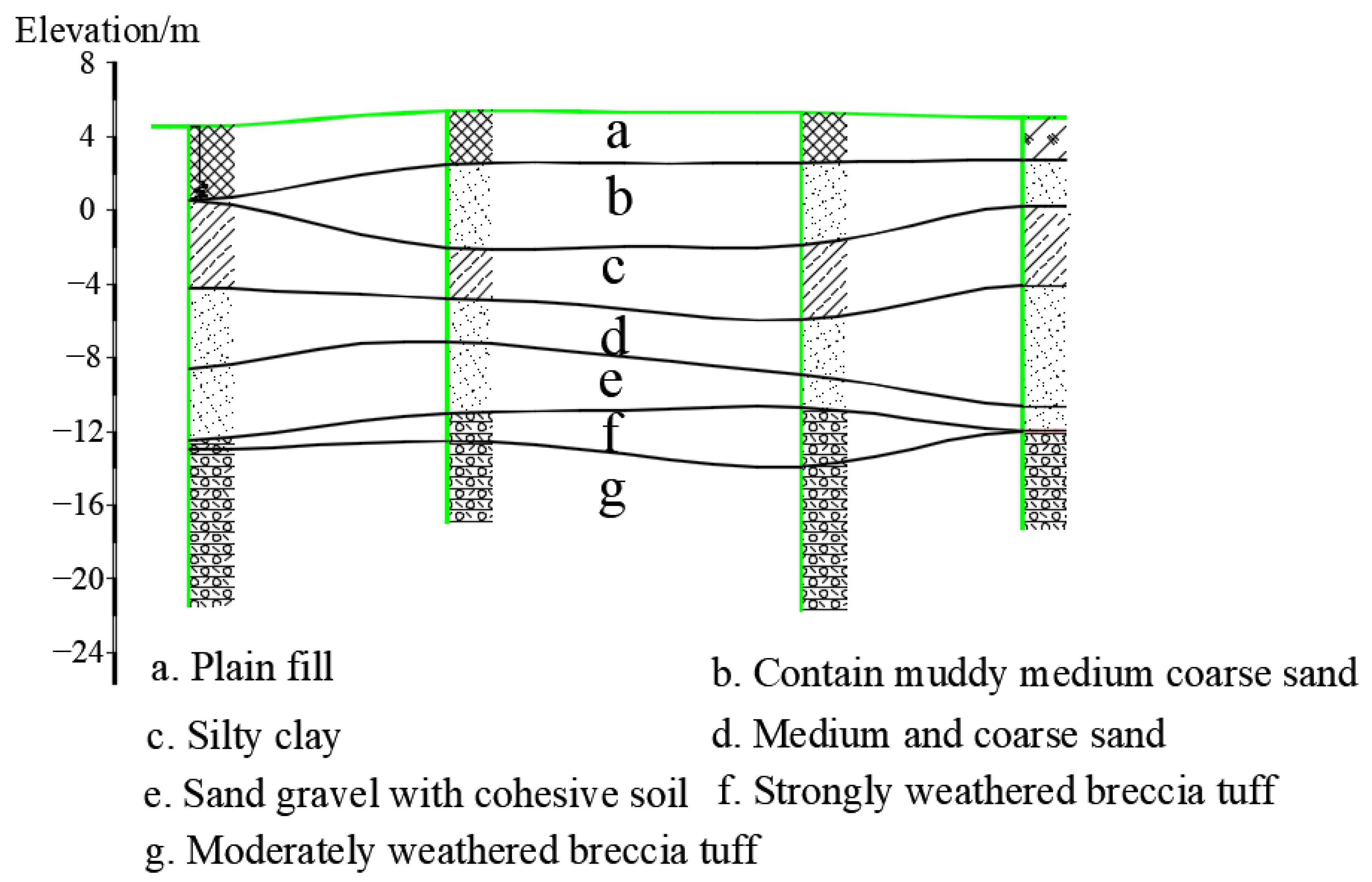
Lingshanwei Station of Line 13 of the Qingdao West Coast Intercity Rail Transit Project is located on the east side of the intersection of Yuewu Road and Taishan East Road and is arranged along Taishan East Road in an east–west direction. The central mileage of the station is YCK14 + 119.1. The design length of the foundation pit is 190 m, the width is 20.7 m, and the excavation depth is 17 m. The geological situation is shown in Figure 1.

The groundwater in the foundation pit site is mainly phreatic water and confined water. The phreatic water is mainly stored in plain fill and contains muddy medium-coarse sand stratum, and the buried depth of the water level is 1~4 m. The confined water is mainly stored in medium and coarse sand and sand gravel stratum.

3.2. Test Plan and Results

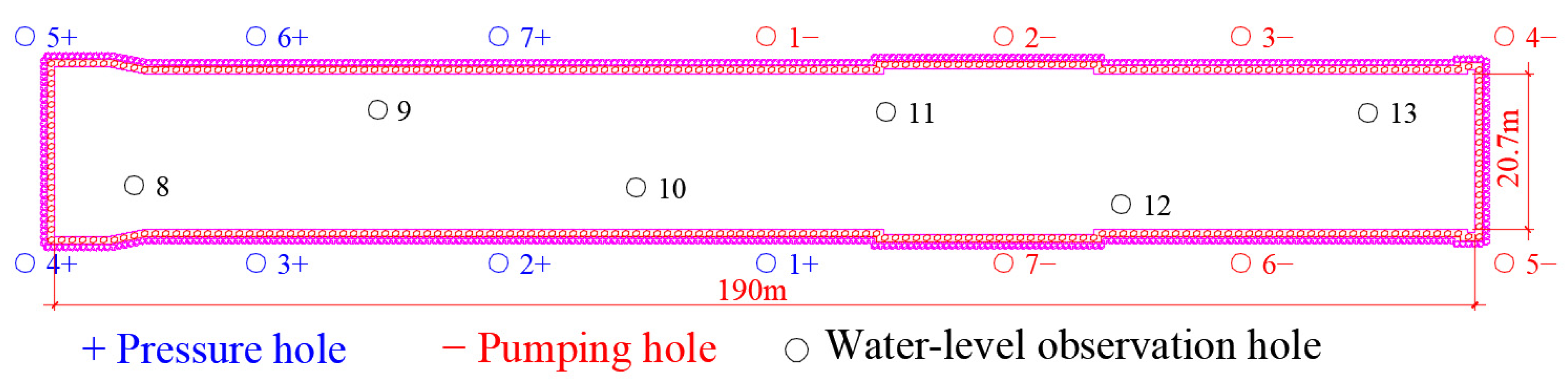
A bored pile was adopted for the foundation pit enclosure structure (φ1000@1200), and a high-pressure rotary jet pile (φ1000@700) was used to check the water curtain. The jet grouting pile is 17~20 m long. To explore the main channels of groundwater seepage in the foundation pit site and the permeability of various strata, water pumping tests were carried out for different strata. There are 14 drillings arranged around the foundation pit and 6 drillings arranged in the foundation pit. The holes around the foundation pit are used as pumping and pressure test holes, and the holes inside the foundation pit are used as water-level observation holes. The arrangement of drilling is shown in Figure 2.

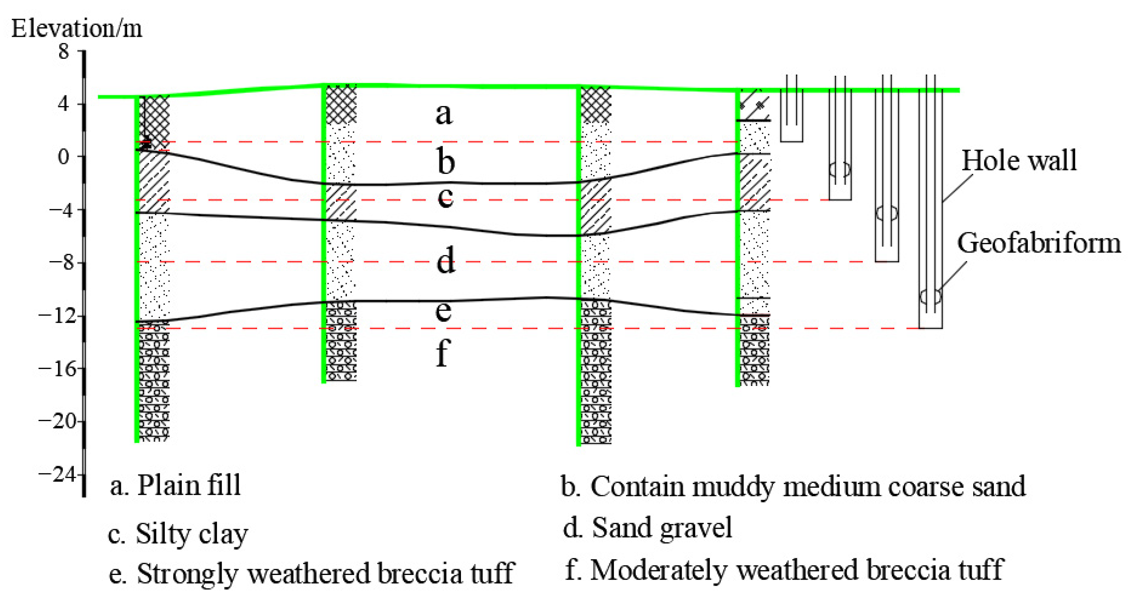
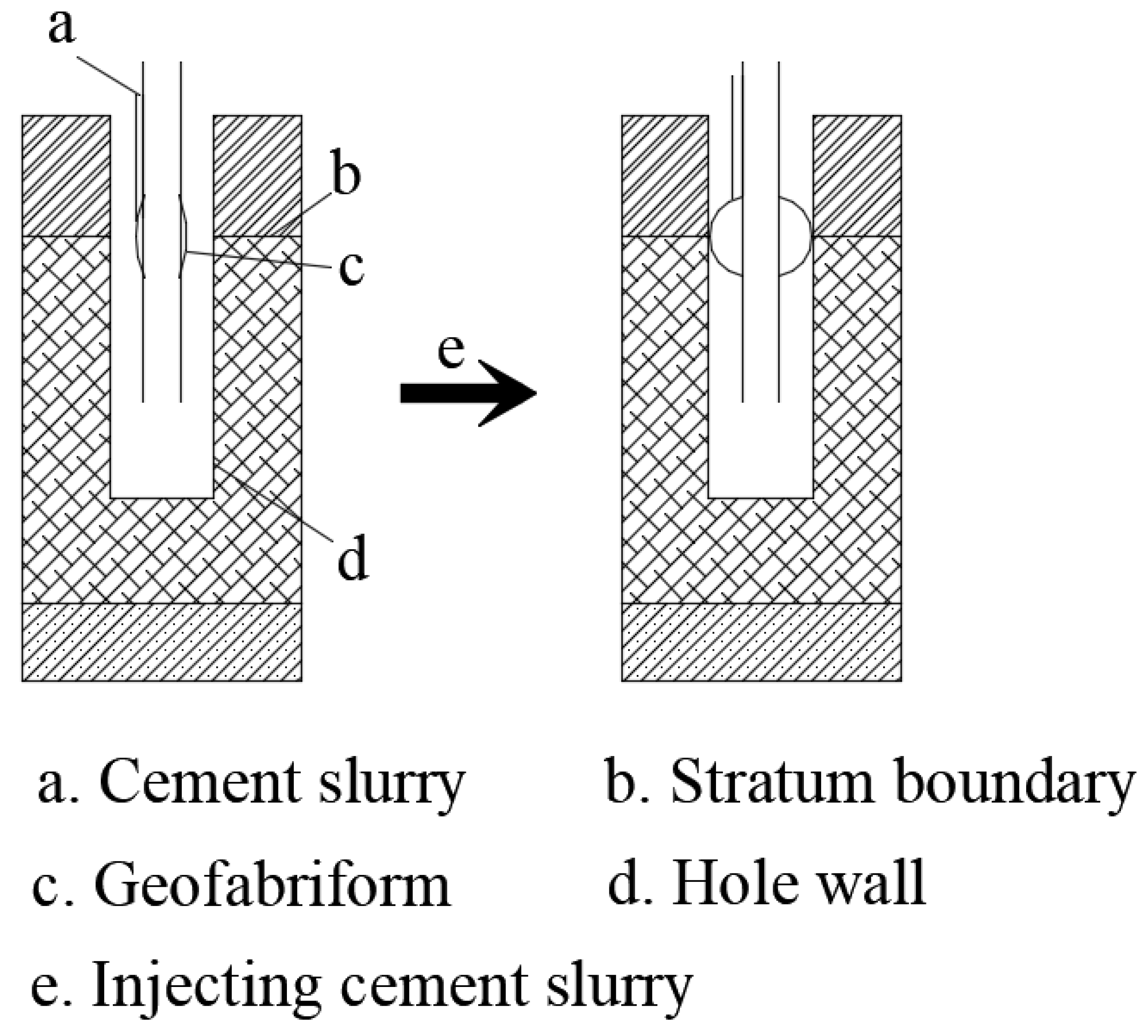
As the aquifer structure of the foundation pit site is complex and strongly water-rich, the excavation site is layered according to the geological type, and the water pumping test is conducted for the contained muddy medium-coarse sand stratum, silty clay stratum, sand gravel stratum, and strongly weathered breccia tuff stratum, respectively. To ensure that each water pumping test only involves the specified stratum, the geofabriform is bound at the stratum boundary of the pressured-water tube. The geofabriform is expanded by injecting cement slurry into the geofabriform, and the drilling is blocked to prevent the water from diffusing to other strata. Taking the midpoint of the stratum thickness as the drilling depth, the drilling depth of each stratum is 4 m, 8 m, 13 m, and 18 m, respectively. The specific drilling depth and testing device principles are shown in Figure 3 and Figure 4.

We carried out seven pumping and water pressure tests at the foundation pit site, respectively. The test plan of pumping water from one hole and pressing water from one hole was adopted for each test. Different strata were pumped and pressed at the same rate (5 L/min). The remaining holes in each test were used as water level observation holes, and their water level changes were recorded. The test results are shown in the following tables (

Table 1. Test data of muddy medium-coarse sand stratum (unit: m).

Test Number	1+	1−	2+	2−	3+	3−	4+	4−	5+	5−
1	Pressure	Pumping	0.40	−0.32	0.23	−0.16	0.10	−0.09	−0.07	−0.01
2	0.09	−0.63	Pressure	Pumping	1.87	−1.29	0.91	−0.81	0.42	−0.64
3	−0.18	−0.57	1.72	−1.44	Pressure	Pumping	2.70	−2.39	1.24	−1.68
4	−0.32	−0.51	0.69	−1.04	2.61	−2.47	Pressure	Pumping	2.67	−2.79
5	−0.47	−0.41	0.20	−0.86	1.14	−1.78	2.68	−2.80	Pressure	Pumping
6	−0.54	−0.35	0.26	−0.99	0.99	−1.75	1.24	−1.64	2.72	−2.36
7	−0.51	−0.14	0.48	−0.96	0.48	−0.84	0.42	−0.60	0.80	−0.73
Test Number	6+	6−	7+	7−	8	9	10	11	12	13
1	−0.19	−0.02	−0.38	−0.06	0.07	−0.13	0.40	−0.44	−0.10	−0.11
2	0.40	−0.86	0.37	−1.06	1.13	1.06	0.81	−1.06	−1.26	−1.01
3	0.98	−1.76	0.27	−1.01	3.28	1.26	0.16	−0.84	−1.71	−3.16
4	1.13	−1.75	0.14	−0.88	3.36	0.63	−0.11	−0.69	−1.28	−3.32
5	2.62	−2.45	0.55	−0.98	2.52	0.94	−0.21	−0.64	−1.37	−2.62
6	Pressure	Pumping	1.43	−1.36	2.42	2.39	−0.13	−0.73	−2.09	−2.18
7	1.61	−1.18	Pressure	Pumping	0.73	2.11	0.21	−0.80	−1.56	−0.81

Note: The number in the title row of the table corresponds to the position of the corresponding hole in Figure 2. For example, “1+” in the table corresponds to the “1+” pressure hole in Figure 2. Each group of experiments is subjected to pressure and pumping in the corresponding holes for “Pressure” and “Pumping” in the table, while the remaining holes are used as observation holes.

,

Table 2. Test data of silty clay stratum (unit: m).

Test Number	1+	1−	2+	2−	3+	3−	4+	4−	5+	5−
1	Pressure	Pumping	1.00	−0.92	0.54	−0.43	0.23	−0.19	−0.22	0.17
2	0.84	−1.08	Pressure	Pumping	2.48	−2.16	1.23	−1.20	0.57	−0.71
3	0.48	−0.49	2.50	−2.15	Pressure	Pumping	2.93	−2.86	1.39	−1.77
4	0.10	−0.32	1.17	−1.26	2.90	−2.97	Pressure	Pumping	2.82	−2.97
5	−0.27	0.12	0.54	−0.75	1.33	−1.83	2.83	−2.96	Pressure	Pumping
6	−0.45	0.52	0.66	−0.74	1.21	−1.70	1.39	−1.70	2.99	−2.88
7	−0.84	0.95	0.92	−0.76	0.76	−0.80	0.61	−0.69	1.20	−1.17
Test Number	6+	6−	7+	7−	8	9	10	11	12	13
1	−0.54	0.42	−0.84	0.95	0.17	−0.35	1.03	−1.02	0.18	−0.19
2	0.60	−0.81	0.89	−0.79	1.56	1.61	1.84	−2.29	−1.85	−1.48
3	1.21	−1.69	0.81	−0.75	3.31	1.78	0.94	−1.01	−2.22	−3.37
4	1.32	−1.77	0.55	−0.75	2.95	1.01	0.41	−0.67	−1.49	−3.24
5	2.94	−2.93	1.11	−1.26	2.57	1.42	0.26	−0.42	−1.17	−2.89
6	Pressure	Pumping	2.33	−2.24	2.65	3.09	0.50	−0.39	−3.12	−2.24
7	2.37	−2.20	Pressure	Pumping	1.11	3.32	1.04	−0.65	−2.72	−0.91

Note: The number in the title row of the table corresponds to the position of the corresponding hole in Figure 2. For example, “1+” in the table corresponds to the “1+” pressure hole in Figure 2. Each group of experiments is subjected to pressure and pumping in the corresponding holes for “Pressure” and “Pumping” in the table, while the remaining holes are used as observation holes.

,

Table 3. Test data of sand gravel stratum (unit: m).

Test Number	1+	1−	2+	2−	3+	3−	4+	4−	5+	5−
1	Pressure	Pumping	0.54	−0.33	0.31	−0.23	0.14	−0.14	−0.03	−0.09
2	−0.26	−1.12	Pressure	Pumping	1.88	−1.05	0.85	−0.72	0.30	−0.61
3	−0.76	−1.30	1.45	−1.48	Pressure	Pumping	2.75	−2.11	1.03	−1.63
4	−0.71	−1.00	0.45	−1.12	2.68	−2.19	Pressure	Pumping	2.54	−2.64
5	−0.72	−0.78	−0.03	−0.94	1.00	−1.66	2.60	−2.58	Pressure	Pumping
6	−0.81	−0.80	−0.04	−1.05	0.67	−1.65	1.13	−1.58	2.65	−2.07
7	−0.65	−0.56	0.12	−0.94	0.21	−0.76	0.32	−0.54	0.76	−0.58
Test Number	6+	6−	7+	7−	8	9	10	11	12	13
1	−0.15	−0.14	−0.32	−0.23	0.10	−0.17	0.56	−0.34	−0.25	−0.18
2	0.14	−0.87	−0.18	−1.23	0.89	0.29	1.11	−1.33	−1.21	−0.88
3	0.48	−1.84	−0.45	−1.42	3.33	0.30	−0.20	−1.43	−1.68	−2.77
4	0.89	−1.82	−0.26	−1.11	3.26	0.34	−0.39	−1.09	−1.31	−3.11
5	2.52	−2.20	0.35	−1.00	2.63	1.22	−0.46	−0.89	−1.21	−2.34
6	Pressure	Pumping	1.32	−1.18	2.60	3.43	−0.44	−1.01	−1.64	−1.96
7	1.64	−0.85	Pressure	Pumping	0.69	2.51	−0.13	−0.91	−1.08	−0.68

Note: The number in the title row of the table corresponds to the position of the corresponding hole in Figure 2. For example, “1+” in the table corresponds to the “1+” pressure hole in Figure 2. Each group of experiments is subjected to pressure and pumping in the corresponding holes for “Pressure” and “Pumping” in the table, while the remaining holes are used as observation holes.

and

Table 4. Test data of strongly weathered breccia tuff stratum (unit: m).

Test Number	1+	1−	2+	2−	3+	3−	4+	4−	5+	5−
1	Pressure	Pumping	0.66	−0.29	0.36	−0.15	0.16	−0.09	−0.08	0.06
2	0.45	−0.50	Pressure	Pumping	2.00	−1.60	1.02	−0.97	0.53	−0.77
3	0.07	−0.44	1.86	−1.73	Pressure	Pumping	2.76	−2.41	1.28	−1.66
4	−0.14	−0.38	0.81	−1.17	2.68	−2.49	Pressure	Pumping	2.73	−2.75
5	−0.35	−0.21	0.29	−1.01	1.16	−1.78	2.72	−2.77	Pressure	Pumping
6	−0.36	−0.01	0.43	−1.21	1.02	−1.84	1.27	−1.63	2.81	−2.49
7	−0.24	0.41	0.77	−1.07	0.64	−0.99	0.54	−0.74	1.01	−1.03
Test Number	6+	6−	7+	7−	8	9	10	11	12	13
1	−0.22	0.14	−0.29	0.36	0.21	0.09	0.96	−0.38	0.05	−0.03
2	0.60	−1.03	0.82	−1.01	1.40	1.51	1.15	−1.41	−1.66	−1.34
3	1.06	−1.81	0.55	−1.10	3.29	1.66	0.45	−0.91	−2.14	−3.06
4	1.20	−1.71	0.35	−0.93	3.34	0.85	0.09	−0.71	−1.53	−2.85
5	2.73	−2.57	0.77	−1.24	2.15	1.08	−0.08	−0.68	−1.68	−2.59
6	Pressure	Pumping	1.79	−1.84	1.87	2.63	0.07	−0.78	−2.51	−2.55
7	1.98	−1.66	Pressure	Pumping	0.77	2.34	0.56	−0.79	−1.91	−1.24

Note: The number in the title row of the table corresponds to the position of the corresponding hole in Figure 2. For example, “1+” in the table corresponds to the “1+” pressure hole in Figure 2. Each group of experiments is subjected to pressure and pumping in the corresponding holes for “Pressure” and “Pumping” in the table, while the remaining holes are used as observation holes.

).

4. The Numerical Calculation Method of Inverse Analysis of the Seepage Field

4.1. Seepage Theory

When there is an aquifer in the rock and soil mass and there is a head difference or flow rate within the aquifer area, seepage is formed. The seepage rate, flow rate, and head changes of groundwater in the aquifer area usually comply with Darcy’s law. The on-site test adopts a constant flow rate test plan of one pumping and one pressure, and the test result is the measured water head change when the water head is stable. It can be considered that the seepage field in the experimental area conforms to Darcy’s law, and the seepage control equation of the seepage field in the experimental area can be expressed as:

$$\nabla \cdot (-{\mathit{k}}_{\mathrm{s}}\nabla \cdot \mathit{H})={\mathit{Q}}_{\mathit{s}}$$

(22)

where $\nabla$ is the Hamiltonian operator, k_s is the permeability coefficient, H is the height of the water head, and Q_s is the source and sinks.

4.2. Principle of Least-Squares Optimization for Back Analysis Models

Assuming (x_i, y_i) is a set of measured values and x = [x₁, x₂, x₃,···, x_n−1, x_n]^T, y = R follows the following functional relationship:

$$\mathit{y}=\mathit{f}(\mathit{x},\mathit{\omega })$$

(23)

Among them, ω = [ω₁, ω₂, ω₃,···, ω_n−1, ω_n] is a pending parameter.

To obtain the function f(x, ω) medium parameter ω based on the obtained m sets of measurement data (x_i, y_i) (i = 1, 2, 3,···, n − 1, n), we must solve the following objective function for the optimal solution.

$$\mathit{L}(\mathit{y},\mathit{f}(\mathit{x},\mathit{\omega }))={\displaystyle \sum _{\mathit{i}=1}^{\mathit{m}}{[{\mathit{y}}_{\mathit{i}}-\mathit{f}({\mathit{x}}_{\mathit{i}},{\mathit{\omega }}_{\mathit{i}})]}^2}$$

(24)

Then, we solve the parameter when Equation (24) takes the minimum value ω_i (i = 1, 2, 3, ···, n − 1, n).

The back analysis model established in this article adopts the L₂ constrained least-squares method, which adds the on-site observation data to the least-squares target physical field of the model. We defined and solved the constrained objective functions using the “optimization” interface in COMSOL Multiphysics 5.6 numerical simulation software. The objective function and constraints are defined based on the components of the control variable and auxiliary variable. The constraint is given as the solution of a differential equation defined by a multi-physical field model.

4.3. Calculation Parameter Setting

The seepage field in practical engineering is a random field varying with the spatial position. In this case, the spatial unknown parameters are infinite, and the measurement results are limited data, so it is difficult to find the unknown parameters. Therefore, the designated test area is discretized as 25 × 4, assuming that the permeability coefficient in each small square element does not change with the spatial position. The model contains a total of 100 unknown parameters. For the seepage field area beyond the test range, the permeability coefficient is set as a constant value [37].

The inverse analysis process is to calculate the permeability coefficient within the test range by using the observations. The precision of water-head measurement in the test ΔH = 1 cm, so the fitness term can be rewritten as:

$$\frac{{‖\mathit{y}-\mathit{f}(\mathit{s})‖}_2^2}{\mathsf{\Delta }{\mathit{H}}^2}$$

(25)

It is assumed that the unknown parameters are isotropic in space. Therefore, the covariance matrix is only a function of the distance of the corresponding points in space, which can be expressed as:

$${\mathit{G}}_{\mathit{i}\mathit{j}}=\mathit{C}(\left|{\mathit{x}}_{\mathit{i}}-{\mathit{x}}_{\mathit{j}}\right|)$$

(26)

A common assumption in the geological sciences is that spatially distributed parameters follow a geostatistical distribution defined by some parameterized variogram. The conventional variogram models are exponential, spherical, and Gaussian. In this paper, the Gaussian variogram is used to calculate the regularization term:

$$\mathit{\gamma }(\mathit{h})=\mathit{C}(1-{\mathit{e}}^{-\frac{{\mathit{h}}^2}{{\mathit{a}}^2}})$$

(27)

The approximate relationship between the variogram and the covariance function [38] is expressed as:

$$\mathit{\gamma }(\mathit{h})=\mathit{C}(0)-\mathit{C}(\mathit{h})$$

(28)

The covariance function can be expressed as:

$$\mathit{C}(\mathit{h})=\mathit{C}\cdot {\mathit{e}}^{-\frac{{\mathit{h}}^2}{{\mathit{a}}^2}}$$

(29)

where x_i is the square centroid corresponding to the unknown parameters, γ(h) is a Gaussian variation function, C is the sill parameter, a is the range, a is also standing as correlation length, and h is the distance between two points in a direction. According to Cardiff [37], the C value is taken as 2 and the a value is taken as 50 m.

To facilitate the calculation, the auxiliary vector u is introduced to further simplify the regularization term:

$$\mathit{\alpha }{(\mathit{s}-\mathbf{X}\mathit{\beta })}^{\mathrm{T}}{\mathbf{G}}^{-1}(\mathit{s}-\mathbf{X}\mathit{\beta })=\mathit{\lambda }{(\mathit{s}-\mathbf{X}\mathit{\beta })}^{\mathrm{T}}\mathbf{u}$$

(30)

$$\mathbf{u}={\mathbf{G}}^{-1}\mathit{(}\mathit{s}-\mathbf{X}\mathit{\beta }\mathit{)}$$

(31)

$$\mathbf{G}\mathbf{u}=\mathit{s}-\mathbf{X}\mathit{\beta }$$

(32)

Since it is often more convenient to solve the value of u in linear Equation (32) than to directly calculate G, the calculation equation of auxiliary vector u is established in the model using domain ordinary differential and differential algebraic equations. Zhou [39] believed that when the λ value is 3, it is the best parameter, which can improve the calculation accuracy of the model. Through the above parameter settings, the observation values can be used for the inverse analysis calculation of the permeability coefficient.

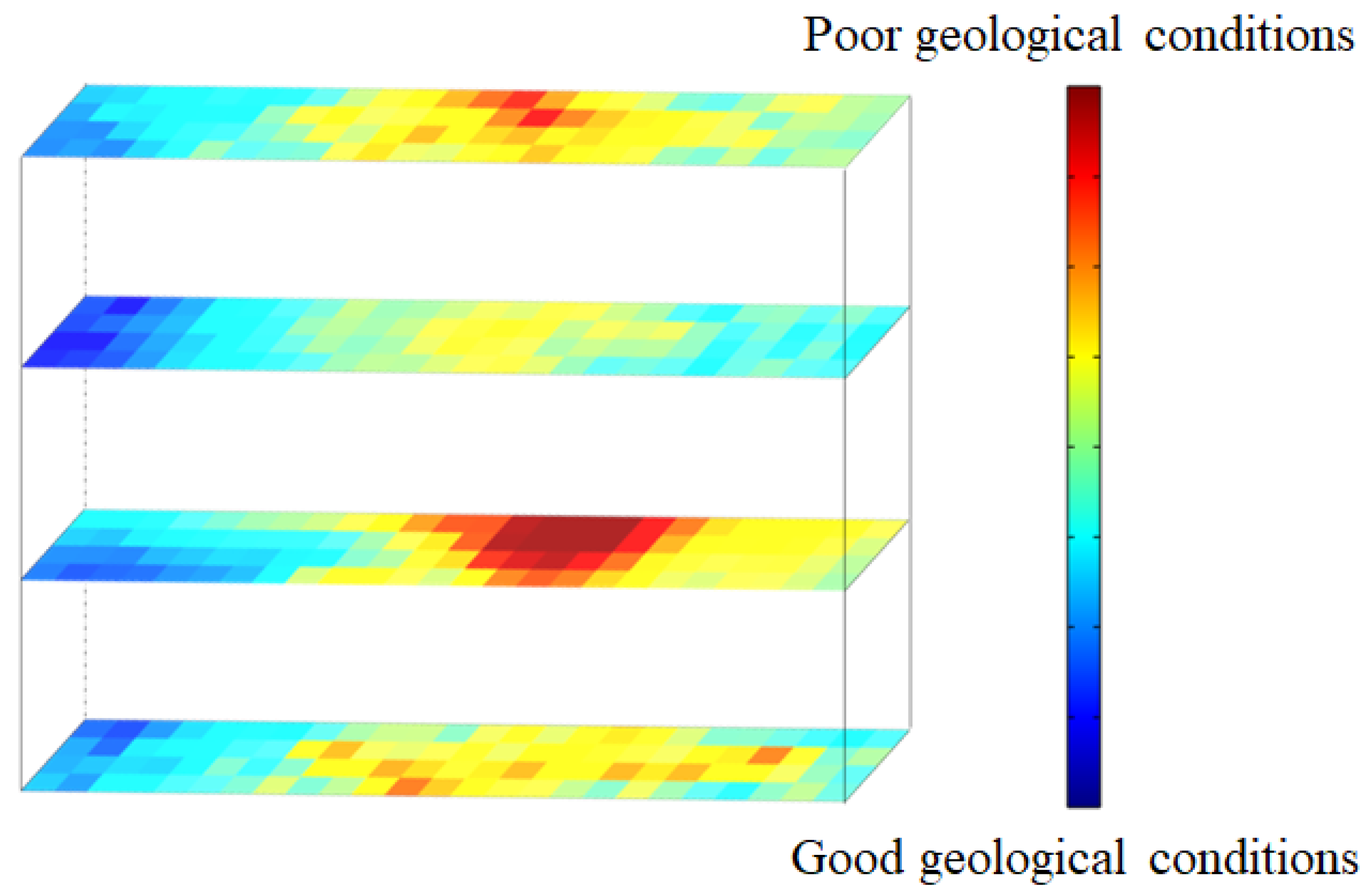
4.4. Numerical Simulation Results and Analysis

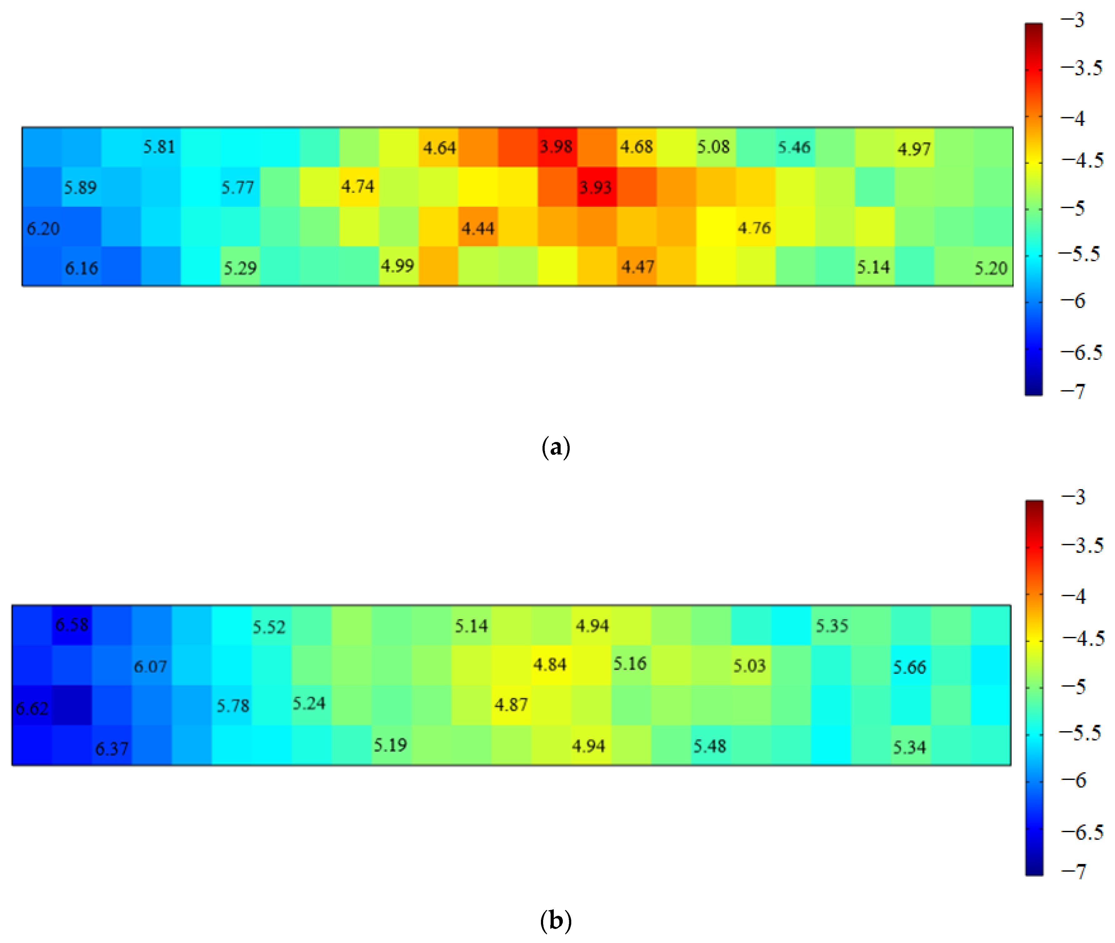
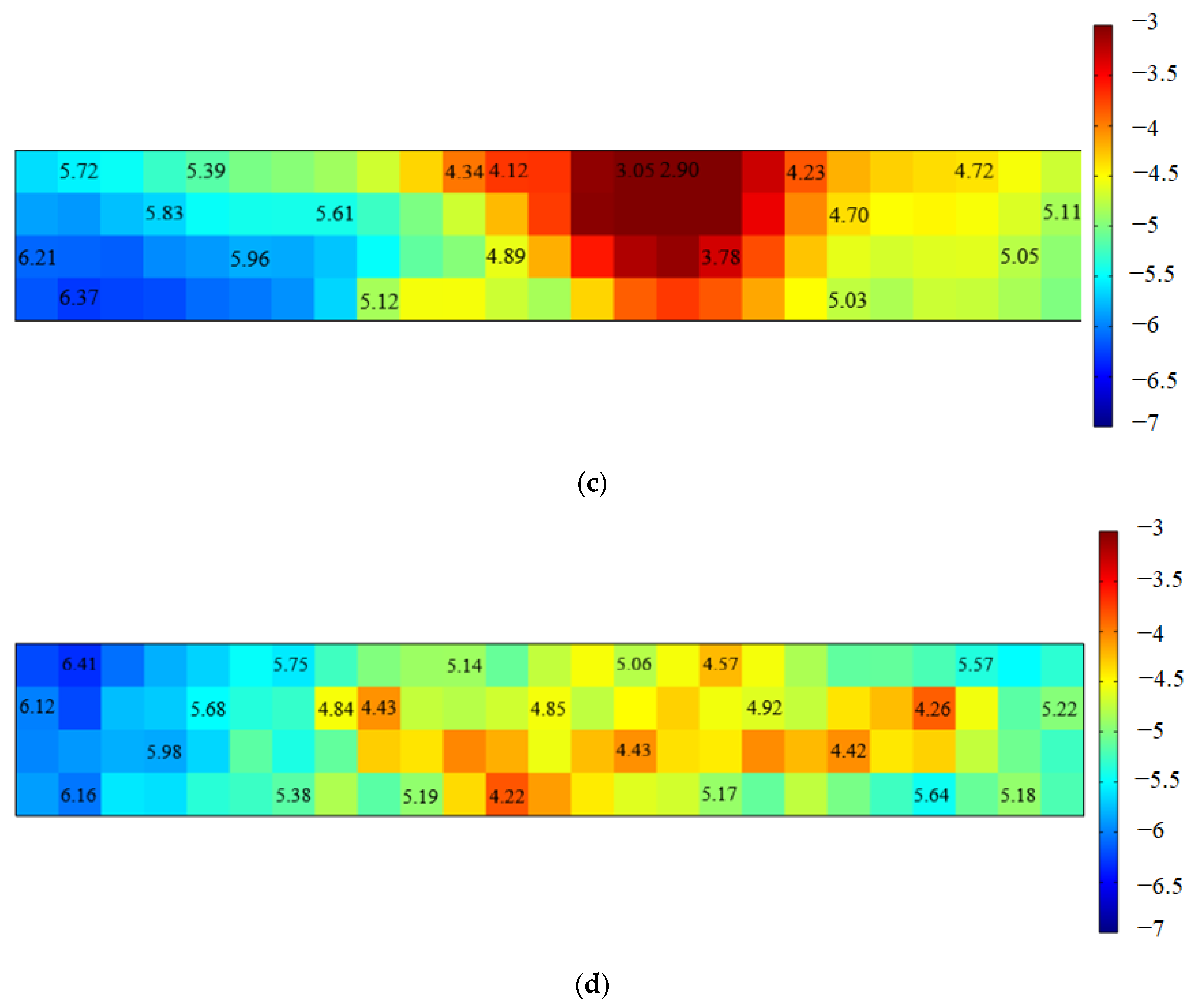
According to the observation values in on-site tests, the permeability coefficients of different strata are calculated based on the inverse analysis calculation model, and the calculation results are shown in Figure 5.

According to the inverse analysis results of different stratum permeability coefficients calculated from the drilling water-head observations, the muddy medium-coarse sand stratum and sand gravel stratum are the broken areas of the stratum in the excavation area of the foundation pit. They have strong water permeability and large water content. Some areas may be connected with groundwater, among which the sand gravel stratum is the most serious. Water gushing or collapse very easily occurs during the excavation process, so such areas should be reinforced and dewatered before excavation. The silty clay stratum has good geological conditions, and its permeability coefficient is mostly 1 × 10⁻⁵ under, basically meeting the requirements of the foundation pit during construction. Although there are broken areas in the strongly weathered breccia tuff stratum, most of them are located in the middle of the foundation pit site, while the permeability coefficient around the foundation pit is small, and only a few places need to be reinforced. It can be inferred that the high-pressure rotary jet pile in the strongly weathered breccia tuff stratum plays a water-stop curtain effect, and it needs to be dewatered before excavation.

5. Comparison and Analysis of Geophysical Exploration Results and Numerical Simulation Results

5.1. Geophysical Exploration

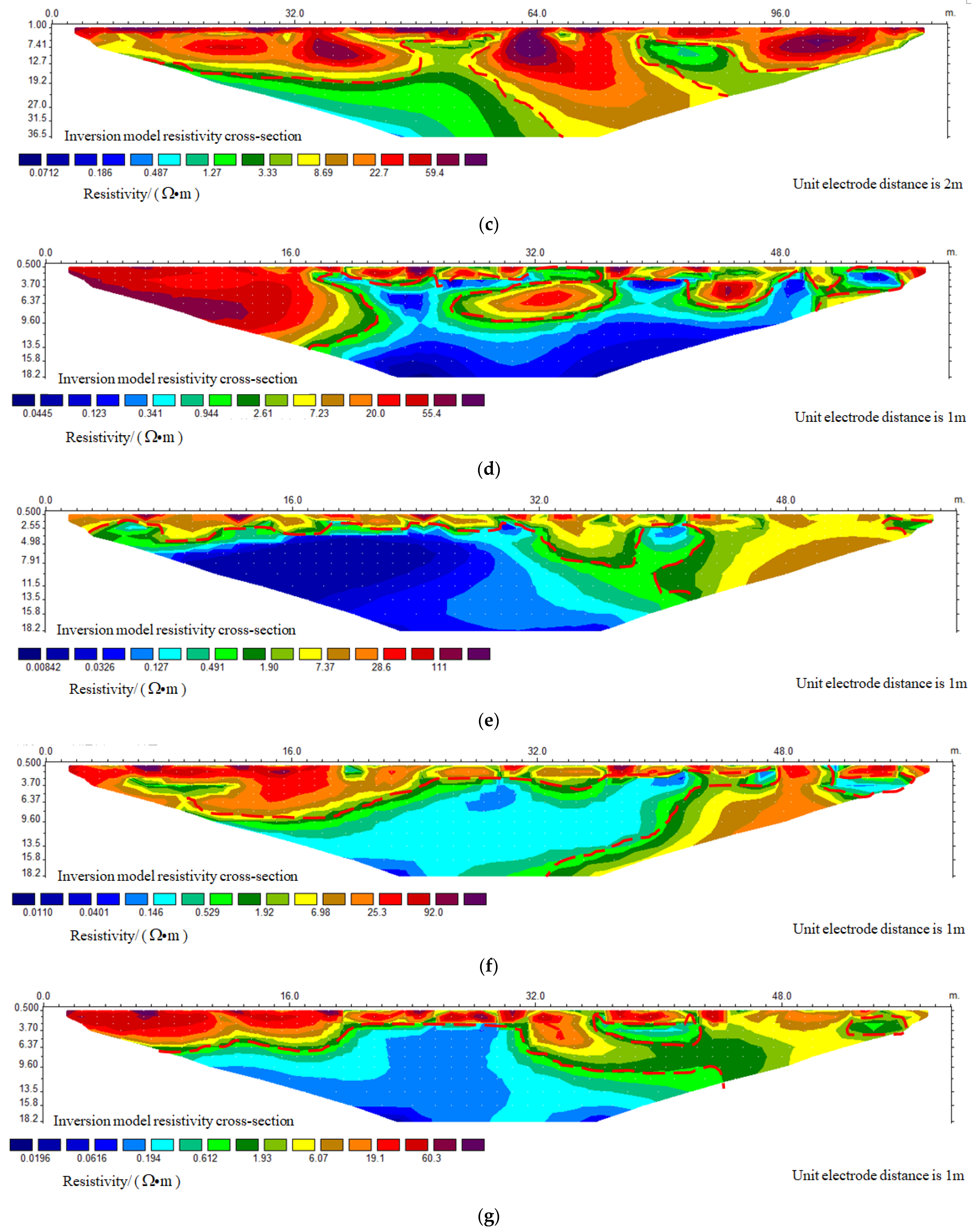
As the aquifer structure of the foundation pit site is complex and strongly water-rich, the geophysical exploration will show an obvious low-resistance area. The multi-electrode resistivity method is used to conduct hydrogeological investigations in the excavation area of the foundation pit. According to the geophysical exploration information of the stratum in the excavation area of the foundation pit, the correctness of the inverse analysis model is verified from the geological situation distribution area.

(1) Multi-electrode resistivity method

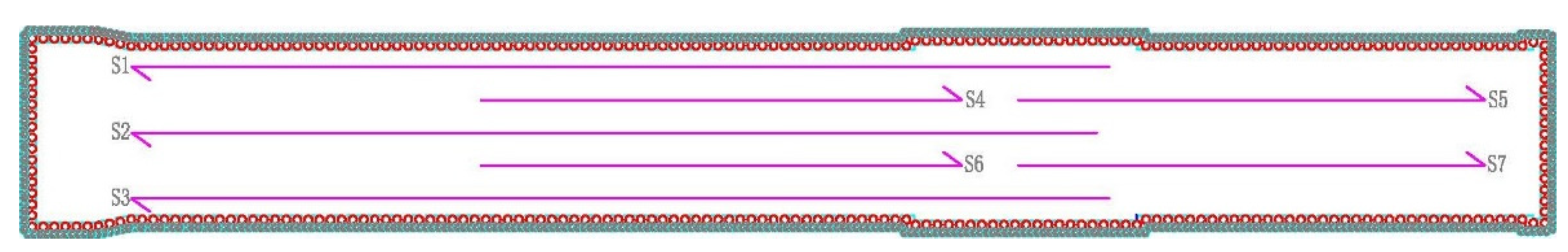
WDA-1, 1 A super digital DC method instrument, and four pole-measurement devices are used for the multi-electrode resistivity method. This detection adopts a quadrupole measuring device with a voltage of 36 volts. The electrode spacing of S1, S2, and S3 measuring lines is 2 m, and the electrode spacing of S4–S7 is 1 m. The measuring lines are arranged horizontally, as shown in Figure 6.

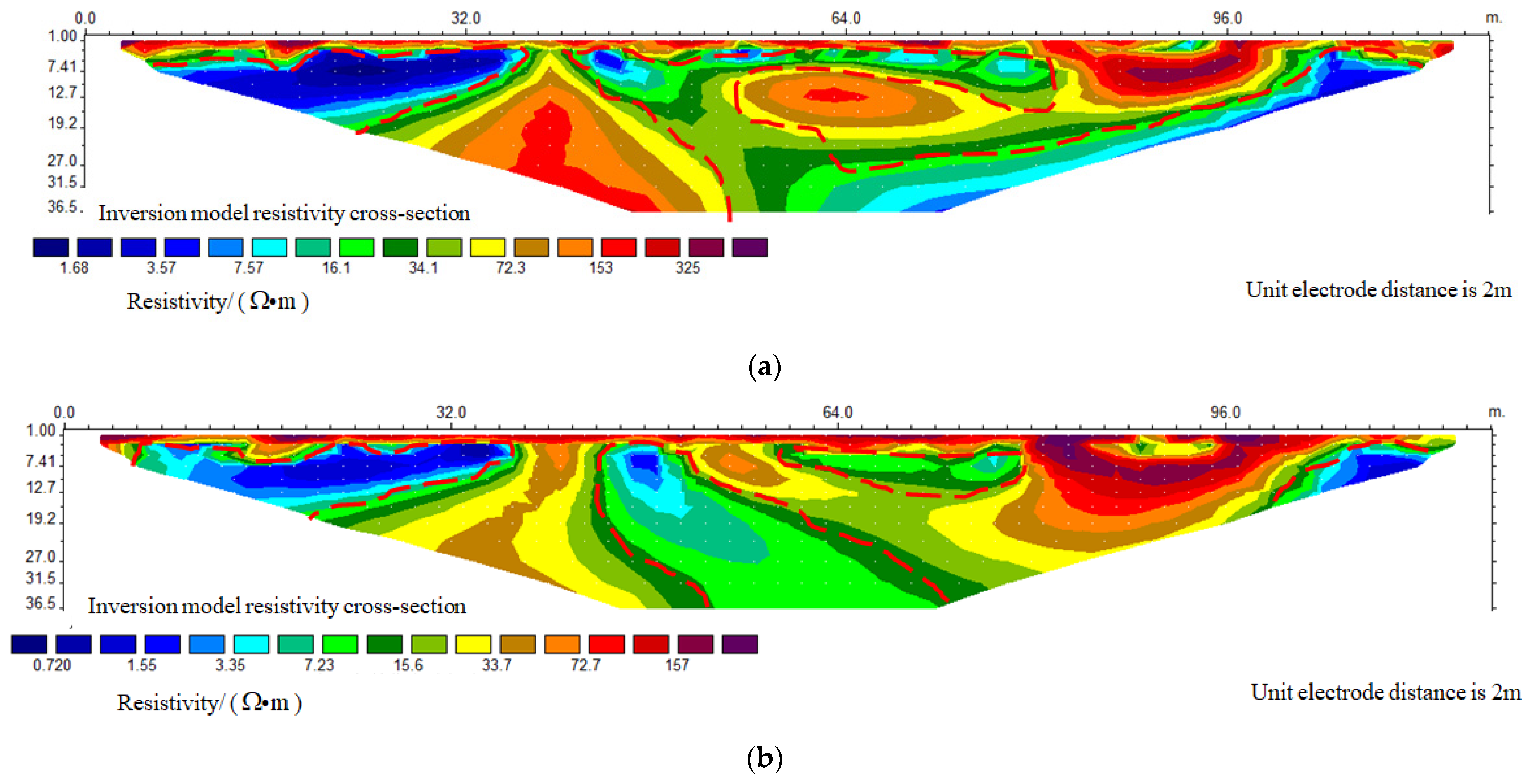
The exploration result is shown in Figure 7, and the marked range is inferred as a water-bearing or mud-filled area.

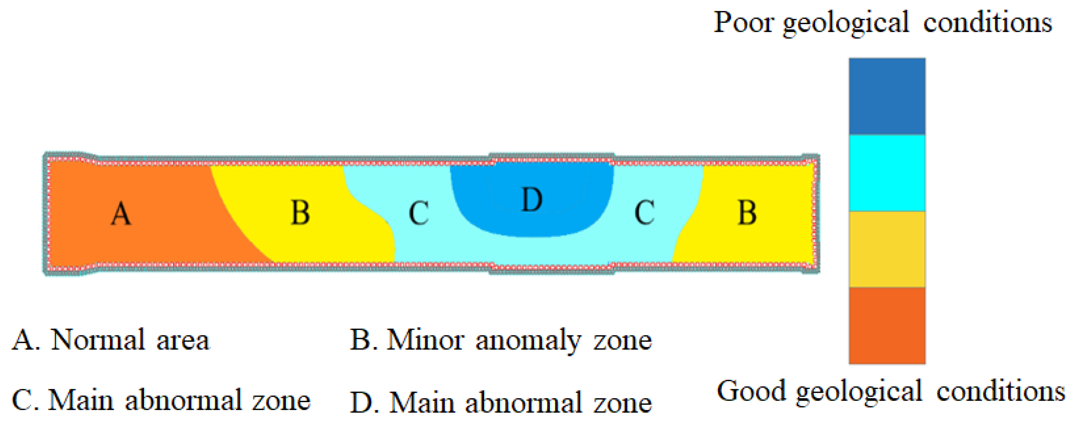
5.2. Analysis of Geophysical Exploration Results and Comparison of Numerical Simulation Results

According to the geophysical exploration results, the distribution of geological conditions in the area affected by foundation pit excavation is shown in Figure 8. It can be seen from the figure that areas C and D are the main abnormal zones. It can be inferred that the geological conditions in this area are poor, the rock mass is broken, the fractures are developed or relatively developed, and the local rock mass is connected with the groundwater. The rock mass in area D is the most broken and the water content is the highest, followed by area C; area B is a minor anomaly zone, and it is inferred that the rock mass in this area is relatively broken and the fractures are relatively developed; area A is a normal area with good geological conditions.

By comparing Figure 8 and Figure 9, it can be seen that the distribution of the permeability coefficient calculated from the on-site pumping and water-pressure test data is consistent with the abnormal location of geophysical exploration, which proves the correctness of the inverse analysis model from the distribution area.

6. Water Injection Test to Test Stratum Permeability

To verify the accuracy of the model calculation results, drilling tests were carried out in the area affected by the excavation of the foundation pit. We used six observation holes (8–13) (see Figure 2) arranged in the foundation pit to conduct the water injection test of the dewatering head, and the permeability coefficients of the contained muddy medium-coarse sand stratum, silty clay stratum, sand gravel stratum, and strongly weathered stratum were measured, respectively. The calculation formula for the permeability coefficient of the water injection test of the dewatering head is [40]:

$$\mathit{k}=\frac{{0.0523{\mathit{r}}_0}^2}{\mathit{A}}\frac{\mathit{ln}({\mathit{H}}_1/{\mathit{H}}_2)}{{\mathit{t}}_2-{\mathit{t}}_1}$$

(33)

where k is the permeability coefficient of the test section, cm/s, r₀ is the inner radius of the casing, cm, A is the shape coefficient, cm, H₁ is the test water head at time t₁, cm, and H₂ is the test water head at time t₂, cm.

See

Table 5. Permeability coefficient of each stratum.

Drilling Number	Contain Muddy Medium-Coarse Sand (cm·s−1)		Silty Clay (cm·s−1)		Sand Gravel (cm·s−1)		Strongly Weathered (cm·s−1)		Error/%
	Drilling Test	Model Calculation	Drilling Test	Model Calculation	Drilling Test	Model Calculation	Drilling Test	Model Calculation	/
8	1.1 × 10−6	1.0 × 10−6	7.7 × 10−7	6.9 × 10−7	6.8 × 10−6	5.8 × 10−6	1.0 × 10−6	1.1 × 10−6	9~17
9	5.6 × 10−6	4.9 × 10−6	2.4 × 10−6	2.9 × 10−6	3.0 × 10−5	2.5 × 10−5	3.7 × 10−6	3.1 × 10−6	14~20
10	1.7 × 10−5	2.0 × 10−5	6.8 × 10−6	5.6 × 10−6	7.3 × 10−5	6.0 × 10−5	3.3 × 10−5	4.0 × 10−5	15~22
11	1.4 × 10−4	1.2 × 10−4	1.1 × 10−5	1.3 × 10−5	8.2 × 10−3	6.8 × 10−3	1.9 × 10−5	1.5 × 10−5	15~27
12	2.0 × 10−5	1.7 × 10−5	7.5 × 10−6	6.2 × 10−6	2.1 × 10−4	2.5 × 10−4	8.2 × 10−6	9.3 × 10−6	12~21
13	6.1 × 10−6	6.9 × 10−6	1.8 × 10−6	2.2 × 10−6	1.3 × 10−4	1.5 × 10−4	1.6 × 10−5	1.4 × 10−5	12~18

Note: Drilling number 8: 9% is strongly weathered, and 17% is sand gravel. Drilling number 9: 14% is medium-coarse sand, and 20% is sand gravel. Drilling number 10: 15% is medium-coarse sand, and 22% is sand gravel. Drilling number 11: 15% is silty clay, and 27% is strongly weathered. Drilling number 12: 12% is strongly weathered, and 21% is silty clay. Drilling number 13: 12% is medium-coarse sand, and 18% is silty clay.

for the test results of the permeability coefficient of the water injection test of the dewatering head.

We analyzed the reasons for the errors in the above table, which mainly come from two aspects. Firstly, there is a certain degree of measurement error in the water injection test. Secondly, the established inverse analysis model also has certain errors, which are caused by measurement errors in the data used, and the established model may also generate errors due to some assumptions.

In the process of water injection testing, to ensure that each water injection test only involves the designated formation, binding the molded bag at the boundary position of the formation may cause certain errors due to the inaccuracy of the instrument and the error of the operator, resulting in a certain difference between the measured formation and the designated formation. The water injection test process will cause disturbance to the formation seepage field, increase the permeability coefficient of the original formation, and cause measurement errors, resulting in the permeability coefficients of most water injection tests in the table being greater than the permeability coefficients calculated by the model. Errors can also occur during measurement due to improper operation by operators, instrument issues, and environmental changes.

In the process of establishing the inverse analysis model, the least-squares method was used to minimize the measurement errors in the on-site test data as much as possible, but measurement errors still exist and will not be eliminated. In underground engineering, geological changes are extremely complex, and it is difficult to accurately predict the geological structure of spatial changes. In most cases, people use averages to describe variables. Using the average value to represent the structural characteristics of the actual seepage field will result in a certain degree of error compared to the actual situation. The seepage field in practical engineering is a random field that varies with spatial position. In this case, the unknown spatial parameters are infinite, and the measurement results are limited data, making it difficult to determine the unknown parameters. By assuming that the permeability coefficient within each unit does not change with spatial position and that the unknown parameter is isotropic in space, the unknown parameter can be calculated, but this can also generate certain errors.

Based on the analysis of errors, it can be concluded that errors are inevitable, but certain actions can be taken to minimize errors as much as possible. For measurement errors, when selecting measurement methods, we can adapt to local conditions and choose appropriate measurement methods; use more precise instruments during the testing process and improve the proficiency of operators; and test under good weather conditions as much as possible to minimize the impact of the environment on the test. For errors caused by spatial variability, a three-dimensional model can be established to study formation permeability, which, to some extent, reduces the impact of spatial variability on errors.

In practical applications, there are often unavoidable variables or situations, making it impossible to achieve absolute accuracy. According to the results of the water injection test, the error between the permeability coefficient by the water injection test and the permeability coefficient calculated by the inverse analysis is about 15%, and the error is within the acceptable range. The injection test results verify the accuracy of the permeability coefficient obtained by the inverse analysis model.

7. Conclusions

The results of this research are as follows:

(1)

Based on the least-squares theory and regularization method, the objective function of an underdetermined inverse analysis problem is proposed. The geostatistical theory and variation function are used to describe the spatial characteristics of the actual engineering system, and a calculation method for the stratum permeability coefficient using the on-site drilling test data is proposed.

(2)

Through the combination of on-site pumping and water pressure tests, on-site drilling test data are obtained. Based on the established inverse analysis model, the permeability coefficient of different strata is calculated. According to the distribution of the permeability coefficient of different strata, the water content and fracture area of each stratum are further determined.

(3)

Geophysical exploration was carried out in the excavation area of the foundation pit. The results show that the distribution of the permeability coefficient calculated by the inverse analysis model is consistent with the plane distribution of geophysical exploration, which verifies the correctness of the inverse analysis model of the stratum seepage field in terms of regional distribution.

(4)

The pumping test was carried out in the affected area of foundation pit excavation, and the results showed that the error between the permeability coefficient calculated by the inverse analysis model and the permeability coefficient by on-site pumping was about 15%, which verified the numerical accuracy of the permeability coefficient calculated by the inverse analysis model.

References

- Qian, Q. Challenges faced by underground projects construction safety and countermeasures. Chin. J. Rock Mech. Eng. 2012, 31, 1945–1956. [Google Scholar]
- Jing, L.; Duan, S.; Yang, S. Application of seepage back analysis to engineering design. Chin. J. Rock Mech. Eng. 2007, 26, 4503–4509. [Google Scholar]
- Li, K.; Deng, X.; He, M.; Chai, J.; Li, S. The establishment of the limited element model based on the penetration coefficient of a tail mine based on drilling data. Chin. J. Rock Mech. Eng. 2004, 23, 4329–4332. [Google Scholar]
- Zhang, X. Pumping test and numerical simulation in an excavation engineering. Geotech. Eng. Tech. 2021, 35, 306–311. [Google Scholar]
- Kitanidis, P.K.; Lee, J. Principal Component Geostatistical Approach for large-dimensional inverse problems. Water Resour. Res. 2014, 50, 5428–5443. [Google Scholar] [CrossRef]
- Bárdossy, A.; Hörning, S. Gaussian and non-Gaussian inverse modeling of groundwater flow using copulas and random mixing. Water Resour. Res. 2016, 52, 4504–4526. [Google Scholar] [CrossRef]
- Yang, J.; Zheng, G.; Jiao, Y. Tianjin Station pumping test numerical inverse analysis. China Civ. Eng. J. 2010, 43, 125–130. [Google Scholar]
- Kitanidis, P.K.; VoMvoris, E.G. A geostatistical approach to the inverse problem in groundwater modeling (steady state) and one-dimensional simulations. Water Resour. Res. 1983, 19, 677–690. [Google Scholar] [CrossRef]
- Kitanidis, P.K. On the geostatistical approach to the inverse problem. Adv. Water Resour. 1996, 19, 333–342. [Google Scholar] [CrossRef]
- Zhang, Z.; Jafarpour, B.; Li, L. Inference of permeability heterogeneity from joint inversion of transient flow and temperature data. Water Resour. Res. 2014, 50, 4710–4725. [Google Scholar] [CrossRef]
- Capriotti, J.; Li, Y. Inversion for permeability distribution from time-lapse gravity data. Geophysics 2015, 80, WA69–WA83. [Google Scholar] [CrossRef]
- Guan, W.; Hu, H.; Wang, Z. Permeability inversion from low-frequency seismoelectric logs in fluid-saturated porous formations. Geophys. Prospect. 2013, 61, 120–133. [Google Scholar] [CrossRef]
- Maqsood, Z.; Koseki, J.; Miyashita, Y.; Xie, J.; Kyokawa, H. Experimental study on the mechanical behaviour of bounded geomaterials under creep and cyclic loading considering effects of instantaneous strain rates. Eng. Geol. 2020, 276, 105774. [Google Scholar] [CrossRef]
- Ojala, I.O.; Ngwenya, B.T.; Main, I.G. Loading rate dependence of permeability evolution in porous aeolian sandstones. J. Geophys. Res. Solid Earth 2004, 109. [Google Scholar] [CrossRef]
- Savvides, A.A.; Papadrakakis, M. A computational study on the uncertainty quantification of failure of clays with a modified Cam-Clay yield criterion. SN Appl. Sci. 2021, 3, 659. [Google Scholar] [CrossRef]
- Savvides, A.A.; Papadrakakis, M. Uncertainty Quantification of Failure of Shallow Foundation on Clayey Soils with a Modified Cam-Clay Yield Criterion and Stochastic FEM. Geotechnics 2022, 2, 348–384. [Google Scholar] [CrossRef]
- Matthies, H.G.; Brenner, C.E.; Bucher, C.G.; Soares, C.G. Uncertainties in probabilistic numerical analysis of structures and solids-stochastic finite elements. Struct. Saf. 1997, 19, 283–336. [Google Scholar] [CrossRef]
- Sett, K.; Jeremić, B.; Kavvas, M.L. Probabilistic elasto-plasticity: Solution and verification in 1D. Acta Geotech. 2007, 2, 211–220. [Google Scholar] [CrossRef]
- Li, D.Q.; Qi, X.H.; Cao, Z.J.; Tang, X.S.; Zhou, W.; Phoon, K.K.; Zhou, C.B. Reliability analysis of strip footing considering spatially variable undrained shear strength that linearly increases with depth. Soils Found. 2015, 55, 866–880. [Google Scholar] [CrossRef]
- Deidda, G.; Diaz De Alba, P.; Rodriguez, G. Identifying the magnetic permeability in multi-frequency EM data inversion. Electron. Trans. Numer. Anal. 2017, 47, 1–17. [Google Scholar] [CrossRef]
- Lee, J.S.; Choi, I.Y.; Lee, H.U.; Lee, H.H. Damage identification of a tunnel liner based on deformation data. Tunn. Undergr. Space Technol. Inc. Trenchless Technol. Res. 2004, 20, 73–80. [Google Scholar] [CrossRef]
- Wang, X.D.; Lv, L.; Shi, J.; Tan, W.J. Weighted multi-curve fitting method for estimating hydrogeological parameters from pumping test. J. Hydraul. Eng. 2020, 51, 276–285. [Google Scholar]
- Cooley, R.L. Incorporation of prior information on parameters into nonlinear regression groundwater flow models, 1, Theory. Water Resour. Res. 1980, 18, 965–976. [Google Scholar] [CrossRef]
- Cooley, R.L. Incorporation of prior information on parameters into nonlinear regression groundwater flow models, 2, Applications. Water Resour. Res. 1983, 19, 662–676. [Google Scholar] [CrossRef]
- Lv, Y.; Wang, S.; Ge, X.; Jiang, H.; Zhang, H. Application of a new global optimization to displacement back analysis for geotechnical engineering. Rock Soil Mech. 2008, 29, 1451–1454. [Google Scholar]
- Zhao, L.L.; Xiao, C.L.; Chen, C.L.; Chen, Z.; Liang, Y. Determination of hydrogeological parameters by a variety of methods based on the pumping test. Chin. J. Undergr. Space Eng. 2015, 11, 306–309+357. [Google Scholar] [CrossRef]
- Du, X.; Zeng, Y.; Tang, D. Research on permeability coefficient of rock mass based on underwater pumping test and its application. Chin. J. Rock Mech. Eng. 2010, 29, 3542–3548. [Google Scholar]
- He, J.; Xu, Q.; Chen, S. Back analysis of permeability of fractured rock. Chin. J. Rock Mech. Eng. 2009, 28, 2730–2735. [Google Scholar]
- Clement, W.P.; Knoll, M.D. Traveltime inversion of vertical radar profiles. Geophysics 2006, 71, K67–K76. [Google Scholar] [CrossRef]
- Wang, J. Inverse Theory in Geophysics; Higher Education Press: Beijing, China, 2002; Volume 27. [Google Scholar]
- Dai, R.; Yin, C.; Liu, Y.; Zhang, X.; Zhao, H.; Yan, K.; Zhang, W. Estimation of generalized Stein’s unbiased risk and selection of the regularization parameter in geophysical inversion problems. Chin. J. Geophys. 2019, 62, 982–992. [Google Scholar]
- Dong, G. The Regularization Method of Inverse Problems and Its Computation. Master’s Thesis, Hunan Normal University, Changsha, China, 2012. [Google Scholar]
- Kitanidis, P.K. Quasi-linear Geostatistical Theory for Inversing. Water Resour. Res. 1995, 31, 2411–2419. [Google Scholar] [CrossRef]
- Zhang, Z.; Zou, Z.S.; Liu, S.C. Geological statistical analysis of the spatial variation law of permeability in karst water-bearing media. Hydrogeol. Eng. Geol. 1995, 22, 4–7. [Google Scholar]
- Liu, S.; Hu, X.; Liu, T. Characteristics and Applications of Variogram for Gravity and Magnetic Fields. Earth Sci. 2014, 39, 1725–1734. [Google Scholar]
- Liu, A.; Wang, P.; Ding, Y. Geostatistics; Science Press: Beijing, China, 2012. [Google Scholar]
- Cardiff, M.; Kitanidis, P.K. Efficient Solution of Nonlinear, Underdetermined Inverse Problems with a Generalized PDE Model. Comput. Geosci. 2008, 34, 1480–1491. [Google Scholar] [CrossRef]
- Zhang, S.; Tang, H.; Liu, X.; Tan, Q.; Xiahou, Y. Seepage and instability characteristics of slope based on spatial variation structure of saturated hydraulic conductivity. Earth Sci. 2018, 43, 622–634. [Google Scholar]
- Zhou, M.; Zhou, S.; Qiao, T.; Chi, Q. An improved method of choosing regularized parameters of penalized least squares. Sci. Surv. Mapp. 2018, 43, 105–108. [Google Scholar]
- Ministry of Water Resources of the PRC. Code of Water Injection Test for Water Resources and Hydropower Engineering (SL345—2007); China Water & Power Press: Beijing, China, 2008.
Figure 1.
Typical section of station geological.
Figure 2.
Schematic diagram of drilling layout.
Figure 3.
Schematic diagram of test hole depth.
Figure 4.
Schematic diagram of the expansion mold bag test device.
Figure 5.
Simulation results of the permeability coefficient of each stratum. (a) Simulation results of muddy medium-coarse sand stratum; (b) Simulation results of silty clay stratum; (c) Simulation results of sand gravel stratum; (d) Simulation results of strongly weathered breccia tuff stratum. Note: The numbers in the figure represent the −lg k (negative logarithmic) value of the permeability coefficient. The legend on the right represents the lg k value of the permeability coefficient.
Figure 6.
Layout of multi-electrode resistivity method survey line.
Figure 7.
Multi-electrode resistivity method exploration results map. (a) S1 survey line exploration results; (b) S2 survey line exploration results; (c) S3 survey line exploration results; (d) S4 survey line exploration results; (e) S5 survey line exploration results; (f) S6 survey line exploration results; (g) S7 survey line exploration results. Note: The range indicated by the red dashed line is inferred as a fractured area of the rock mass, containing water or filled with mud.
Figure 8.
Geophysical exploration results plan figure.
Figure 9.
Distribution of the permeability coefficient of each stratum.