

Kinesthetic Learning Based on Fast Marching Square Method for Manipulation


Robotics Lab, Universidad Carlos III de Madrid, 28911 Leganes, Spain
*
Author to whom correspondence should be addressed.
Appl. Sci. 2023, 13(4), 2028; https://doi.org/10.3390/app13042028
Submission received: 21 December 2022
/
Revised: 31 January 2023
/
Accepted: 2 February 2023
/
Published: 4 February 2023
(This article belongs to the Special Issue Advances in Intelligent Control and Engineering Applications)
Abstract
:The advancement of robotics in recent years has driven the growth of robotic applications for more complex tasks requiring manipulation capabilities. Recent works have focused on adapting learning methods to manipulation applications which are stochastic and may not converge. In this paper, a kinesthetic learning method based on fast marching square is presented. This method poses great advantages such as ensuring convergence and is based on learning from the experience of a human demonstrator. For this purpose, the demonstrator teaches paths by physically guiding one of the UR3 arms of a mobile manipulator. After this first phase, the fast marching Learning method is used to make the robot learn from this experience. As a novelty, an auto-learning functionality is presented, which provides the kinesthetic learning algorithm with an exploration capacity. The base of this algorithm is not only using the information provided by the taught trajectories, but also expanding its ability in order to explore unknown states of the environment. The effectiveness of the proposed method has been evaluated through simulations in 2D and 3D environments and in a real mobile manipulator. The learning process is analyzed with other 2D learning approaches using the LASA dataset and it is tested in complex 3D scenarios with different obstacles, proving its effectiveness.
1. Introduction
In today’s robotics, the need for precise manipulation has encouraged the development of human-like robots. This has led to the emergence of manipulator arms of all kinds of shapes and configurations in order to achieve a system capable of reproducing natural human-inspired movements. To guarantee this similarity, robotic arms have a large number of degrees of freedom (DoF). For this reason, path planning and control for these platforms have become a very difficult task [1]. The most common way to solve this kind of problem in robotics is to use inverse kinematics. However, redundant manipulators carrying out complex tasks hinder classical methods from successfully solving this problem.
The most common way to overcome this is based on the use of different learning methods. Learning algorithms would obtain a policy that works in a similar way as a human does. The main objective of these strategies is to identify patterns and then try to generalize the more relevant features for the given data. With that information, the algorithm tries to reproduce new behaviors resembling previous learned experiences, even if there is a change in the environment of the study or if it is unknown. When applying these methods to manipulation, the concept of learning in complex manipulating tasks lies in the use of knowledge taught by a human who shows how to solve a task and the generalization of that information for similar tasks [2,3].
Traditional learning methods have shown good performance for the resolution of manipulation problems [4,5]. However, the process needed in those methods to obtain the learning policy generates a mathematical model which usually relies on probabilistic terms, which makes these learning methods stochastic. Depending on what would need to be solved, this characteristic may not be a desirable property, since even with the same demonstrations, different solutions could be obtained in each test. This stochastic behavior may cause algorithms to end up obtaining a solution that does not converge.
In this paper, we propose a learning-based solution that overcomes typical problems from both traditional planners and learning methods. It is an extension of a previous work proposed in [6,7], which focuses on the generation of trajectories for a robotic manipulator for tasks in two dimensions and without the use of imitation learning techniques. We present the fast marching learning (FML) method, which is a deterministic and asymptotically globally stable learning algorithm created for learning point-to-point 2D and 3D tasks based on the fast marching square () method [8,9]. The proposed learning approach is either referred to in this work as fast marching learning or as learning based on the fast marching square.
Initially, paths are kinesthetically taught to the robot by guiding its robotic manipulator. Then, these trajectories are represented by , which is a path planner based on how the light propagates. This treats the environment where it is applied in a continuous way, deriving multiple benefits which will be discussed later. FML applies on every learned path to parameterize experience, which is later merged for obtaining a global knowledge representation. Additionally, some relevant optimizations are made with respect to our previous publications and a new concept of auto-learning is presented herein. A direct relation between the proposed method and common learning techniques, such as reinforcement learning (RL), is also carried out. Finally, a large amount of testing trials on a real robotic manipulator are performed to fully validate the functioning of the proposed strategy in 3D complex indoor environments. Regarding the state-of-the-art techniques and the previous work presented in [6,7], the following advantages were obtained:
- The generated trajectories are ensured to be smooth and local minima-free, which means that these always converge.
- The path planner method is complete. If there is any solution, it is always found.
- The proposed approach can handle high-dimensional data and it can learn from one or more demonstrations.
- The method presents an ability to explore unknown environments even if it has not been taught beforehand, searching for the fastest paths. In addition, this exploration allows one to work on dynamic environments where objects that were not accounted for during data acquisition are present.
- It can guarantee a correct performance regardless of the variation of starting points even in the case of high-dimensional complex motions.
- It is robust against erroneous paths learned during data acquisition.
- The method overcomes state-of-the-art methods in terms of similarity with respect to demonstrations.
- The method improves on previous works because it can be applied to a real robot, makes use of kinesthetic learning techniques and can be applied in both 2D and 3D.
The work presented in this paper is focused on the use of a specific learning method known as learning by imitation [10], which is also referred to as programming by demonstration (PbD) [11]. In this type of learning, the robot is provided with a set of demonstrations as input. These demonstrations can be given in different ways, including by observing human demonstrators doing a task, collecting data by haptic devices and physically guiding the robot to emulate the task that must be learned (i.e., kinesthetic teaching). When dealing with learning by human demonstration, motion capture (MOCAP) suits are usually the preferable option, as highlighted in [12]. This methodology is based on marker point measurements from a 3D motion capture system. However, it requires the system to deal with the re-targeting problem, since robotic arm joints do not necessarily have the same structure as the human arm. Regarding haptic learning, there are different options that can be developed. One of the most common ways consists in the use of some haptic device which may be similar to a joystick [13] that the user controls to generate training data. Other common ways to work with the haptic method are based on the use of a twin master to capture data [14]. Typically, that twin master is a simplified version of the robotic arm, which is provided with a sufficient amount of sensors to capture the required data and to report the user through haptic information on any problem that may occur. Another important detail is that those devices normally have the same structure as the real arm, which eliminates the re-targeting problem. However, these haptic-based method have some drawbacks. Given the great amount of DoF of manipulator arms, it may not be intuitive to operate these devices through just a joystick. In case of using a twin master, possible delays between the twin and the real arm movements could also occur, which could lead to delays in data collection or even potential collisions when performing complex trajectories. Kinesthetic teaching solves all these problems.
First of all, as for the demonstration (data collection) and reproduction of the learned movements, the same embodiment is used: the real robot. Hence, the re-targeting problem does not appear and furthermore, no delays in the data acquisition process exist. Second of all, data collection is performed in an very intuitive way by moving the robotic arm through the desired positions. This process generates point-to-point trajectories, which will be used as input for the learning algorithm. When performing kinesthetic teaching, two different types of tasks can be identified. Firstly, there are tasks where the path does not necessarily require critical accuracy. In those kind of tasks, the main objective is not to move to a specific point but to perform a certain controlled dynamic in the movement. This type of task focuses on teaching the robot how to complete a given task without any data about the initial or goal position. Examples of these kinds of missions include ability games taught to the robot, like the ball in a cup game [15,16] or the work in [17], where a robot learns how to play table tennis using a variety of simple motor tasks which represent just elementary actions. The most common way to solve these learning tasks is by using dynamic motion primitives (DMP) [18,19]. The main idea is to teach simple functional movements that can be combined and adapted to solve new and more complex tasks. Based on this idea, reinforcement learning techniques are found in the literature to carry out this learning process of primitives [20,21]. Even though these methods are helpful for the above-mentioned applications, this paper is focused on manipulating objects in a certain location. Hence, the followed trajectories are not initially optimized with respect to distance, requiring additional steps.
The second type of task that can be performed for motion learning are known as point-to-point tasks. In this case, a specific goal state is given while the initial state may vary. The aim for this type of motion learning is to teach the robot how a discrete motion is performed. Hence, this is the learning type in which our work is focused. In order to face this problem, different approaches in the literature are found and reviewed. Some works propose the use of gradient techniques for point-to-point task learning. The authors in [22] defined an extension of the Maximum Margin Planning (MMP) [23]. The algorithm, called LEARCH (Learning to Search), uses gradient descent techniques to learn the cost map given the training paths, which were generated by an expert. The strategy tries to imitate the expert policy by performing regression upon features from paths using support vector regression (SVR) and iteratively updates the map with that knowledge. This map is then used to plan the needed path for the task through any path planning algorithm. The Unified Motion and Variable Impedance Control (UMIC) technique was presented in [24]. It defines a control policy to regulate both the robot movement and its dynamic interactions with the environment. The main objective is to encapsulate the potential function gradient and the curvature in the same model so that motions resemble the learned path while respecting the velocity profile taught in the demonstration. It is time-invariant and the learning process can be carried out based on a few demonstrations by solving just two constrained quadratic optimization problems. However, the main issue of using gradients is that there is a risk of deriving into local minima. The authors in [25] proposed the stable estimator of dynamical systems (SEDS), which constraints the Gaussian mixture regression model parameters to learn globally stable motions. One of the main issues from this method is that strict constraints limit the learning accuracy from taught data. In [26], the algorithm named control Lyapunov function-based dynamics movement (CLF-DMs) is presented. Initially, a roughly consistent Lyapunov function is learned with respect to taught data, which is used for deriving estimated motions using regression techniques. Stability is then ensured solving a constrained convex optimization problem. The work presented in [27] proposes the FSM-DM method based on extreme learning machine to consider three factors when learning: stability, accuracy and learning speed. Even though results from the three methodologies are promising, there are two main drawbacks: none of them are applicable to high-dimensional spaces and they do not work with a single demonstration.
Other techniques are better-suited for three-dimensional spaces. The authors in [28] proposed a kinesthetic teaching approach based on Motion Primitives (MP) and Gaussian Process Latent Variable Models (GPLVM). Initially, the paths are kinesthetically taught to a robot with the help of an operator. In order to model these learned paths, MP group motion trajectories that present time-dependent variances over time and their dimensionality is reduced with GPLVM. The resulting latent space is finally mapped into a reward for the learning algorithm. In [29], a neuronal network is proposed for the learning procedure, obtaining a better reproduction performance while guaranteeing the generalization ability. This method (modified DS) has several limitations derived from the use of neural networks as can be the great amount of parameters that need to be controlled for the training time. Overall, the main issue of all these presented kinesthetic learning methods is that they are highly dependent on taught trajectories. New paths calculated using acquired knowledge strictly follow learned data. There might be cases in which it could be useful for learning methods to have the ability to explore new trajectories. This is key in situations such as having corrupted learned data or having a single demonstration. The Fast Marching Learning method proposes an auto-learning factor to combine the usage of learned data and the exploration of unknown regions.
The rest of the paper is organized as follows. In Section 2, the Fast Marching Square method is explained, with special emphasis on its implementation in the path planning problem. In Section 3, the FML method is presented by giving an in-depth account of kinesthetic data collection explaining the auto-learning process developed, explaining the ability to add obstacles and making a direct comparison with the RL structure. Section 4 presents a series of experiments in both two and three dimensions performed to test the benefits of the developed method. For this purpose, a handwriting human motion dataset created by LASA has been used for the empirical comparison of the method developed for two dimensions. In the case of three dimensions, a series of tests were carried out in an indoor environment, both in simulation and in a real environment using a robotic manipulator. Section 5 presents the final conclusions and proposes future work.
2. Fast Marching Applied to Path Planning
The Fast Marching Square (FM) method [30] is a path planning algorithm which is a variation of the original Fast Marching Method [31]. It is based on the idea of guiding the desired path by following light propagation. Mathematically, light propagation is defined by the Eikonal equation, which states that the speed of light is determined by the substance in which it is travelling [32]. This equation is solved by the solution of wave propagation, as stated in Equation (1):
where and represent the wave value and initial wave value, respectively, is the refraction index and is the light speed. According to this definition, some properties of the proposed method can be derived:
- The path that light follows is always the fastest feasible one, so the proposed planning method ensures the calculation of the path of least possible time.
- Given the characteristics of Equation (1), if is , then is also , and so are the calculated trajectories using the gradient method over this potential. This turns into smooth paths that avoid the need for extra refinement steps.
- Since the method is based on wave propagation, if there is a feasible solution, it is always found, so it is complete.
Following its original definition, fast marching solves the Eikonal equation applied on a rectangular orthogonal mesh, deriving into a algorithm where n is the total number of grid points. The discrete formulation of the Eikonal function can be seen in Equation (2):
where and are the grid spacing in the x and y directions, is the wave propagation speed for the grid cell (i,j) and T represents the arrival time of the Eikonal equation for each position. If this time T is represented for the different values and , it is obtained that:
where T sets the time in the current cell and the values of and set the minimum values of the time in the neighboring cells previously visited to the current cell by the expansion of the Eikonal equation. Iterations of the propagation procedure on a grid can be visually observed in Figure 1.
The final outcome is a matrix where each cell indicates the arrival time of the wave with respect to the propagation point. As a modification of FM, applies this procedure twice, deriving in safer and smoother paths. This path planning method () can be applied to binary maps by propagating a wavefront that consider all obstacles as source points. The final matrix is considered as a velocity map . To better show the differences between FM and , the paths are calculated on a sample binary map and shown in Figure 2 and Figure 3. Both figures show that the path obtained with the FM method is smoother and reproducible by a robot.
The velocity map values range from 0 to 1, representing the maximum speed allowed for the vehicle at each point of the map. Obstacles imply speeds equal to zero, whilst points in space far enough from obstacles will allow maximum speeds. When computing a path for the vehicles to follow, the FM method will obtain the shortest path from the initial position to the goal position that lets the vehicles navigate at greater speeds. On the other hand, the original FM method will compute the shortest path, not taking into account the safety of the vehicle. Assuming that contains relative velocities between 0 and 1, it is possible to trim (saturate) this velocity map. With this small modification, the safety and smoothness of the computed paths is still ensured (except for saturation values close to 0), while obtaining trajectories closer to the optimal one in terms of distance. Examples are shown in Figure 4. It is also possible to saturate the map based on a safety distance from obstacles. That is, instead of using an index between 0 and 1 to saturate the map, we can directly set a distance in cells from where the velocity will be 1 (safe for the vehicle). We call this parameter the area of influence (aoi). If each cell corresponds to a square meter, an aoi of five cells corresponds to a security distance from obstacles of 5 m. Examples are shown in Figure 5.
3. Learning Manipulation Trajectories via Fast Marching Square
The main idea of using Fast Marching Square (FM) for learning is to take advantage of the benefits of this path planner. One of its greatest advantages is its capacity to guide planned paths through places of the environment in which the propagation velocity is higher. This generates that the total path can be covered in less time. Consequently, one of the main ideas in the use of this method for learning is to force generated paths to take a similar direction as learned paths. Following this concept, the method tries to exploit learned data to generate similar paths. To do that, the method amends the F matrix so that learned data obtained via kinesthetic teaching will have faster values in the matrix. Other advantages that arise from the use of FM are its smoothness and being local minima-free.
In this paper, we are focused on point-to-point tasks in which we teach the robot different trajectories for the manipulation of elements of the environment. Once these trajectories are available, they are codified as point sequences in the workspace. By generalizing these paths, similar paths can be generated for any specific task. Therefore, the application of FM generates more efficient results that the ones generated by just applying kinesthetic teaching, making faster and smoother paths. Figure 6 shows the three proposed steps for performing learning based on Fast Marching Square. First, data are kinesthetically collected. Then, Fast Marching Learning is applied to acquire knowledge from provided data. Finally, new paths are generated considering an additional auto-learning process, which includes the capacity of finding new unexplored paths. These processes are hereunder described in more detail.
3.1. Kinesthetic Data Collection
The FML algorithm needs learning data generated by a user as input. To prevent the problems presented in Section 1, such as re-targeting, data collection is directly performed with the robot itself. The data acquisition process, therefore, is based on kinesthetic learning, where the user moves the ADAM robotic arms generating the trajectories required for the task to be performed. This robotic platform is presented in Figure 7.
The arms used for this project are UR3 from the Universal Robots company. This arm is an ultra-light and compact collaborative industrial robot, with a weight of 11 kg, a payload of 3 kg and a rotation of ±360 for the first five joints and infinite rotation at the end-effector. To facilitate the process of taking data with the arm, two grips have been designed at the critical control points of the arm, namely the end-effector and the elbow, as shown in Figure 8. These grips allow the user to have greater control of the six joints, thus allowing the generation of trajectories to be much more natural and similar to those that a human would perform.
These elements can be easily removed from the robot after kinesthetic teaching has been carried out and they can be used on both arms. With these grips, the user can handle the arm in a simple and controlled way, as shown in Figure 9, where the person can handle the last three joints through the end-effector grip (gray), and the first three joints through the elbow grip (green).
For path generation, an algorithm with a constant time cycle T has been designed. This algorithm allows to store the position in Cartesian coordinates of the end-effector. Therefore, each of the paths P that are taught will contain a set of N points in the three-dimensional space conformed by p(x,y,z). Since this method has been created for its use in real environments, it has been established that more than one path can be taken to teach the robot. Therefore, K different paths can be made, which will make up the robot’s experience E that can be codified as
where each path consists of
Although data collection may seem trivial, it is a very important step and must be performed correctly in order not to generate errors that can be accumulated during the learning step. Empirically, it has been found that there are two preferable ways to collect data. The first one is to perform a movement at a very low speed, having full control of all the joints of the robot. The second one is to perform a path at a high speed, in which, due to the inertia of the movement, the transmission of any possible disturbance from the person teaching the trajectory is avoided. Figure 10 shows results from gathering data in three different ways, where the same path has been taught using different strategies depending on the velocity and stability.
As shown in Figure 10, results are clearly better in cases where the user has full control of the robotic arm. When using low velocity and a full control of the 6DoF of the arm, correct paths are generated but with a greater amount of points than in other cases. If the user decides to use a high velocity demonstration, the path generated has less points than in the previous case, but the path precision is reduced compared with the low-velocity case. Therefore, there is no single way to solve the kinesthetic learning task. It has been empirically proven that, for precise tasks, it is better to perform a teaching process at low speed and have control of all the DoF, and for more general tasks, it is better to use a teaching process at high speeds. In addition to this, a combination of both forms of data acquisition can be carried out, performing a high-speed data acquisition for approaching the end point and then performing a low-speed control to increase the accuracy of the task.
Regarding data acquisition, a code was developed with which, by using ROS, the values of the joints are read and stored in a path. Subsequently, a filtering process is performed, where we avoid possible repeated points due to the sampling rate and perform the relevant transformations to go from a reference point at the base of the arm to a reference point at the base of the robot. As such, we can apply FML and directly send movement commands to the real robot.
It is important to emphasize that, although filtering for duplicate point removal is necessary, small perturbation removal is not required. This is because the paths will be used as a basis for learning, but applying the FM method will provide the method with some of its advantages, directly obtaining smooth paths as an advantage with respect to those paths used for traditional learning.
3.2. Fast Marching Learning Algorithm
Fast Marching Square, as mentioned previously, creates a velocity map in which a path is optimal when the propagation velocity is higher. Hence, by modifying these velocities, the final calculated path can be reshaped. This fact is very useful for the learning step. Given a set of experiences, the main objective of Fast Marching Learning is to encode this information into the velocity map. As such, the final path would be biased by learned experiences without losing the main properties of Fast Marching Square, such as avoiding local minima and being smooth.
The proposed algorithm takes as inputs the point-to-point paths from the robot’s end effector learned with kinesthetic teaching, defined with Equations (4) and (5). As an output, it is intended to replicate the shape of learned paths when a similar task is commanded. Given that the outcome is based on learned experience, the final path is expected to be efficient, smooth and faster.
The first step is labeling all the points contained in E as 1 in an empty workspace, that is to say, filled with 0. The resulting workspace is denoted as . Then, a dilation operation is applied on . The dilation size is defined by the area of influence (aoi), specified in voxels in the case of 3D environments. After the dilation process is applied, the workspace is divided into regions filled with 1, where previous knowledge is found, and other zones with 0, where no information is available. For the latter ones, the algorithm works as FM normally does.
When the workspace is ready, Fast Marching is applied in the same way as in the first step for FM, turning the workspace into a velocity map. is linearly rescaled to be within the established bounds , where stands for , which is in charge of weighting the importance of new data with respect to the rest of the environment. With this, the final velocity map is obtained. This leads into a generalization in of the provided demonstrations. Finally, Fast Marching is applied on the entire workspace considering a unique wave source defined by the centroid of all final trajectory points and the velocity map . A detailed description of the algorithm coding is shown in Algorithm 1.
| Algorithm 1 Fast Marching Learning Algorithm. |
|
3.3. Auto-Learning Process
The use of kinesthetic learning generates a series of advantages over other learning methods, such as computation speed, since it is based on a series of data taken by an expert, or the generation of paths or movement orders in which there are no collision problems. These ideas are based on the use of the exploitation of known information as a means to generate optimal and fast results. When working with learning methods in robotics, it is very important to find a balance between the use of already learned data (exploitation) and the acquisition of new data autonomously (exploration) [33]. Without exploration, the FML method will always return to the first learned path, and better paths will never be found. On the other hand, if the FML method explores too much, it cannot stick to a path, performing different paths each time, which does not generate real learning.
There are different strategies for balancing exploration and exploitation, which allow a choice to be made between a process of exploitation of prior knowledge and the generation of new data through exploration. One of the most commonly used forms is the -greedy method, in which a small probability is responsible for selecting the best action or generating a random option to encourage exploration. Another form to work with this is the use of Boltzmann selection, where the probability that an action will be selected depends on how it is compared with other action values. In order to obtain such a balance in FML, the FM applies its characteristic of always obtaining the fastest path. When kinesthetic learning is carried out, a modification of the matrix is forced, thus generating a series of tunnels or routes which the method will use for the estimation of ideal paths. It may happen that, when FM is applied, it estimates that to go from one point to another, there is a faster path than the learned one. If only the exploitation of the obtained learning is used, it will be forced to obtain a similar path to those learned, which in this case will generate a non-optimal path. Therefore, in order to encourage exploration, an extension of FML has been generated. An estimation of the obtained path is made and a learning process is carried out so that the new obtained path, which is better than previous knowledge, is also learned. As such, an auto-learning process is generated with which the robot, through exploration, increases its knowledge of the environment. In order to be able to control when auto-learning takes place or when FML makes use of the exploitation of learned information, it is necessary to establish similar criteria to those explained above. For this purpose, a selection strategy has been created based on the coincidence of the generated path with the kinesthetically learned paths. Given a new path, the velocity values on the matrix for each of its points are checked. In zones where the new path is outside the kinesthetic learned paths, very low velocity values close to 0 are found, whereas for those zones within the learned paths, high velocities close to 1 are present. Following these facts, the selection strategy is defined according to Equation (6).
where is the auto-learning factor, is the value of the velocity matrix for a point of the path and l is the length of the evaluated path. Based on the value of , auto-learning will be applied or not. This threshold was empirically obtained by calculating the mean values for different trajectories using only the kinesthetically learned values, so that through various tests, it was established that if the value of , it can be estimated as a new learned path, and therefore, it will be added to the previously taught paths. An example of the application of the auto-learning method with respect to the value is presented in Figure 11.
As in the -greedy method, the value obtained as the optimal threshold is not mandatory for the implementation. Depending on the strategy to follow, the user can decide to work more conservatively, encouraging the use of learned data (decreasing the value of the threshold) or encouraging the addition of new paths obtained (increasing the threshold).
The application of auto-learning is highly beneficial in FML oriented to manipulation for two cases in particular. The first is that, by having the ability to learn and add such automatic learning to previous data, it is not necessary to teach all possible cases of a workspace. As such, by teaching the robot the most common cases so that it can generalize and by having the auto-learning method to be able to learn more specific cases, almost all the activities to be carried out in a given workspace can be covered. This also ensures that no segregation of data arises. This means that there is a possibility that the robot is only taught to perform one type of movement (e.g., downward movements). With auto-learning, the robot can learn other types of movements, such as lateral movements, thus generating a series of new paths that have not been taught in a kinesthetic way.
Secondly, the use of auto-learning allows the correction of possible errors in data collection. If incorrect data acquisition is performed, in which movements that are impossible for the robot to perform are generated, auto-learning will avoid carrying out those erroneous paths and it will permit to learn correct paths to perform the required task. An example of both cases can be seen in Section 4.2.
3.4. Important Parameters: Saturation and Area of Influence
In the FML method, there are two parameters derived from Fast Marching that are essential for the correct behavior of the algorithm, which are saturation and area of influence.
Saturation () represents the propagation velocity of FM. Saturation in FML is used to indicate the places with previous experience or auto-learned experience. Therefore, places that have previous experience will be reached earlier. If the saturation value is really low, the method will only use the experience provided for the kinesthetic data. On the contrary, if the value is very high, the method will encourage the exploration of the environment by not following exactly learned values.
The area of influence () allows to estimate the dilation of the path points in order to give connectivity to the demonstrations and its spatial surroundings. In two-dimensional environments, the area of influence is in pixels (px) and in three dimensions it is measured in voxels (vx). This parameter affects the learning generalization. When an excessively low value is given, the algorithm will not generalize and it will strictly follow the taught trajectories. In the opposite case, the reproductions will excessively generalize and the demonstrations shapes will be lost. Normally, this parameter usually follows a morphologically flat structural element based on a disc, which allows the dilatation processes to be carried out according to the value of the selected aoi, as shown in Figure 12.
In the proposed case, where we are working in three dimensions, both for the FML process and for the cases where auto-learning is necessary, a multidimensional structure has to be applied (in this case in three dimensions). When working with 2-dimensional elements, as shown in Figure 12, it may happen that areas that have been auto-learned do not appear as traversable areas for the algorithm. This is due to path orientation changes. If the path is totally parallel to the base where we are taking data, the disc will be dilating parallel to the ground. Therefore, non-passable areas between auto-learned zones are created due to the lack of the third dimension (height) of the structure, obtaining a result in which a totally unconnected path is obtained. An example of this can be seen in Figure 13 where the result of the same auto-learning is compared using a typical 2-dimensional structure (disc) and a 3-dimensional structure (sphere).
It can also be seen that the use of 3D structures does not only improve the regions that are parallel to the ground, but also that a positive influence is achieved for the curved paths, as shown in Figure 13.
3.5. Addition of Obstacles in the Workspace
Real environments are rarely completely free and are usually dynamic. This is why obstacle inclusion is necessary. Obstacles can belong to the environment from the beginning, which allows the robot to be taught to take them into account, or they can be added later once kinesthetic learning has already taken place. Due to the advantages of FML and FM, both cases can be solved in a simple way.
If the obstacles in the environment are initially known, the solution is trivial because the kinesthetic teaching will take these obstacles into account, thus generating paths that allow the obstacles to be circumvented. An example of this case in 2 dimensions is shown in Figure 14.
In the case of initially having a free environment (), the learning process will be carried out without taking into account any obstacle, generating a certain experience E, which will have a velocity map F associated with it. As soon as any obstacle appears dynamically, it will be necessary to create a new velocity map , which will be saturated. For this work, we considered a dynamic object as one that, after having learned a series of trajectories, appears and interferes with previously learned data. In other types of algorithms, where only the information that has been learned is used and there is no exploration, this type of situation requires either a new learning procedure of the modified environment, or systems for detecting and processing this type of situation. In the presented algorithm, the auto-learning process through the use of exploration determines a new path that is able to avoid the dynamic object. After verifying its feasibility, the new plan is added as a learned path, thus extending the knowledge of the environment as well as accelerating the process in case the object remains in that position. As such, to obtain the final velocity map, it will be necessary to apply Equation (7) to all the points in which is not saturated.
That process has to be repeated any time a new obstacle appears in the environment. The method is the same for 2D and 3D. An example in two dimensions of the dynamic appearance of an object in a free environment can be seen in Figure 15 with and .
An example of the process in three dimensions is represented in Section 4.2.
3.6. Fast Marching Learning Characteristics
Due to the characteristics derived from FM, there are a number of advantages which make it possible for the FML to solve problems that may arise when it comes to learning.
3.6.1. Deterministic Behavior
Since FM is a deterministic method, FML is also deterministic. This means that, when using FML, we will obtain the same output (path) as long as the input is invariant. This factor can be important because it allows the behavior of the generated trajectories to be known and therefore avoids erratic behavior that could cause damage to the robot, which is common in probabilistic methods.
3.6.2. Bi-Directional Behavior
Other learning methods are designed in such way that they can only generate solutions in one direction, i.e., from the start point to the end point. In case of needing a trajectory going in the opposite direction, from the end point to the start point, a totally new and unexpected behavior would be generated. In the case of FML, the same movement learned to go in one direction is applied to return in the opposite direction. Although it can be assumed as a limitation, it allows the method to predict the robot’s behavior, thus increasing the safety when working in environments with humans, as well as ensuring that, in both cases, the fastest path is obtained.
3.6.3. Behavior with No Previous Experience
In other learning algorithms, having a point away from learned experience generates erratic and unpredictable behavior. In cases where there is no prior information, the FML method will obtain the fastest path from the starting point to the end point, always according to the metric obtained from the velocity matrix. Due to the use of a constant saturation () value at points far from previous experience or where there is no previous experience, the fastest path also means the shortest path in terms of distance and time. An example of the application of such behavior is represented in Figure 16, where a path without previous experience (no kinesthetic data) and a path with previous experience (kinesthetic) have been created.
3.6.4. One-Shot Learning
As described in [34,35], one-shot learning refers to the characteristics that some learning methods have to be able to successfully reproduce and generalize certain tasks with a single taught demonstration. This is a relevant and important feature, as it allows a reduction in the amount of data to be collected, which can reduce to a certain extent the errors derived from the difficulty that this sometimes entails.
When a large number of kinesthetic demonstrations are applied in the FML method, in the dilation stage, the algorithm tends to generate a single area of influence, where, depending on the set, more or less demonstrations can be grouped together. Therefore, what the method establishes is a single demonstration derived from the union of many demonstrations. The union of several learned tasks makes it possible to generate a single area of interest larger than with a single learned path, but which behaves as a one-shot learning. An example of the application of one-shot learning in two dimensions is represented in Figure 17.
3.6.5. Stable Behavior
Fast Marching Learning has been proven to be stable according to an analysis based on the Lyapunov Stability Theorem adapted to non-dynamical systems [7]. Equation (2), defining wave propagation, is considered as the Lyapunov function . It starts at the specified goal for the robot, where . Given that the propagation values are based on the wave arrival times, no negative values can be found. Additionally, as distance increases from the initial point, the values of also increase. Finally, since no local minima are found in and given the increasing value of the wave, the derivative of the function is always positive.
Added to the above facts, when the gradient is applied on the function, it descends following the direction in which time decreases the most. Hence, the Lyapunov conditions are met, proving that the system is asymptotically stable. This means that every motion calculated with FML converges to the same point, since only a single minimum exists in .
3.6.6. Limitations of the Method
The main disadvantage of FML derives directly form the disadvantages of FM. The main problem is given by the high dimensionality of the working environment. Working in environments where the search space is very high or the resolution is very small results in an excessively large working matrix, which makes the FM method unable to obtain a solution in a reasonable time because the equation must check a large number of points. This problem is often encountered when working in outdoor environments where large navigation areas have to be covered for trajectory planning with mobile robots or UAVs [36]. To avoid this problem in robotic manipulation, a constant environment matrix value is set. This matrix will have as maximum and minimum range the values of the manipulator workspace and the minimum resolution possible. In our case, a working matrix of cells with a resolution of 1 cm is established.
3.7. Fast Marching Learning as a Reinforcement Learning Problem
As explained in previous sections, robotic arm control for environmental elements manipulation needs to have a balance between tasks that we give to the robot and tasks that it can learn autonomously. The generation and use of the FML method is based on the application of the general characteristics of reinforcement learning algorithms [37], where the robot is supposed to take different actions in an environment so as to maximize the value of a specific cumulative reward, but obtaining the advantages of the FM method for the generation of the trajectories. Specifically, the developed algorithm establishes a direct relationship of its structure with Markov Decision Processes (MDPs) [38]. In MDPs, the robot selects an action a in a given state according to a specific policy created , which tries to maximize a reward function r provided that there is a transition probability of being in state after selecting an action when in state . MDPs are generated using the idea that the actions and states are finite. Thus, the task to be solved can be easily defined as a sequence of different behaviors given descriptive state variables. A schematic of the MDPs is represented in Figure 18.
Despite the advantages of MDP, working with this method in manipulation with a large number of DoF is not trivial. Due to high dimensionality, a large number of actions can exist as a function of states, which leads to an infinite number of state–action pairs. The FML algorithm manages to solve this problem due to the direct application of FM, that allows working in a discretized space obtaining results in a continuous space. As such, FML allows working in a priory environment with infinite actions (continuous), simplifying the positions of the end-effector to a discrete space and subsequently obtaining a sequence of actions for each state. If we relate the elements established for the MDPs to the direct application using FML on the robotic arms, we obtain that the actions are denoted by the actions to be performed by each motor. States allow us to represent each of the joint and end-effector positions. The control policy, when working with FM, will be denoted by the potential matrix which represents the arrival times at the specified points. As this policy will always seek to minimize the distance and time to perform a task, which entails seeking the maximum combination of velocities, it can be assumed that the reward for the FML is represented by the velocity matrix. Positive reinforcement is obtained for going through the fastest and more favorable areas (without obstacles). Negative reinforcement will be given for the slower and less favorable areas (areas closed to obstacles). This control policy therefore allows the position commands to each motor to be estimated on a state-by-state basis. In this case, the obtained policy is deterministic.
Unlike in FM, where a direct estimation is made between the initial and final points, thus obtaining the path to follow, in FML, this process is carried out for each of the points that make up the path between the initial and final points. As such, the action of the next state is obtained only taking into account the previous state as well as the decisions taken in it.
4. Experimental Evaluation of FML Algorithm
To evaluate the performance of the proposed method, different experiments have been made. The first experiment is based on the replication of different handwriting paths generated by the user. For that experiment, the LASA human handwriting dataset [39] is used. It contains thirty recorded handwriting motions that were generated using a Tablet-PC, and is commonly used as a benchmark to evaluate different algorithms and its performances, as explained in [24,40]. With this experiment, the algorithm capability to solve complex motions in two-dimensional environments is shown.
The second experiment is based on different three-dimensional tasks developed for the six DoF UR3 arm in a real environment. This experiment is divided in multiple tasks to prove the ability of the method to solve real daily assignments that can be performed in an indoor environment with and without obstacles (that can be static and dynamic). Through this experiment, it is demonstrated how the method allows the safe execution of a task while being able to precisely dodge the different elements of the environment.
4.1. Experiments Based on Human Handwriting Paths
Recorded motions in the LASA human handwriting library are two-dimensional, i.e., . For each generated pattern, seven demonstrations are provided, where the starting motion point is represented by different initial positions and the ending position is the same point in all cases. All the provided demonstrations have the same number of data points and may intersect with each other. Among the 30 handwriting motions in the library, 26 of them include one single pattern that represents one-shot-learning examples. Three of them are formed by two patterns and one by three patterns, representing multiple-shot-learning examples. For this experiment, it has been decided to make use of some predetermined and constant values for all the tests. As such, it is possible to see how the method works without being affected by a variable change. For this experiment, a and were taken as starting data. The experiment in two dimensions is divided into two different cases. The first case is used to compare the developed method (FML) against a group of methods from state of the art without taking into account the auto-learning process. This will allow verifying how well the generated paths fit learned data. The second case will compare the results, taking into account the auto-learning process, which allows one to evaluate the advantages of the algorithm in terms of trajectory optimization and speed. Figure 19 and Figure 20 show the result of using FML in the LASA dataset. In Figure 19, the result of using the method without using the auto-learning process can be seen. In this case, there is no environment exploration so the method perfectly follows the data learned by demonstration. Figure 20 shows the method using the auto-learning process. As it is shown in this sub-figure, the method generates an optimization in path length and the time to solve the different cases. Overall, the figures show how reproductions (blue lines) closely match demonstrations (red points) when the auto-learning is not working, and when this process is working, the method has the ability to obtain correct paths in which the execution time is shorter. This promotes the developed algorithm having a balance between the exploration of the environment and the exploitation of learned data. In addition to the obtained values, several tests have been performed with variations in both the saturation and size of the area of influence, obtaining always satisfactory results for saturation values between
Once results have been presented qualitatively with the LASA dataset, a quantitative comparison has been made with some of the most widely used algorithms in the state of the art for the trajectory generation using learning methods (presented in Section 1). Those algorithms are SEDS, CLF-DM, FSM-DM, UMIC and Modified DS, whose source codes are all available online. Their characteristics are presented in Table 1.
For this process, a quantitative comparison was made using two error functions: swept error area (SEA) [26] and velocity mean square error [41]. The SEA equation is defined as follows:
where corresponds to the area of the tetragon generated by the four points represented as , where and indicate the sampled points in the trajectory reproduced by the method and the demonstrated trajectories, respectively. To visually understand the equation, an explanation using schematics is shown in Figure 21. can be computed following the next equation:
where represents the velocity of the trajectory generated by the learned method and represents the velocity of the trajectories in demonstrations, where 0 means that the velocity of the method generates a response as fast as learned data.
Therefore, the SEA score can be understood as the error in the reproduction of a learned path, comparing the shapes between learned demonstrations and the generated path for each method, while measures the preservation of the velocities of the demonstrated motions. A comparison of between the results of the FML method and the other selected methods is presented in Table 2.
As expressed in Table 2, FML has clear advantages over the other methods. The mean SEA has a lower value, which means that it has a better reproduction when keeping the same starting points. FML also has a lower value, which means that reproductions are as smooth as demonstrations, which is one of the previously presented advantages. When FML used auto-learning, the SEA error cannot be used because, due to the path optimization of the FML, a shorter path length is obtained, which does not allow a point-to-point comparison with the kinesthetically acquired data. Therefore, only can be used. FML with auto-learning achieves a lower velocity due to the resulting path length reduction, as previously represented in Figure 20. Thus, it can be observed that shorter paths generate faster responses. FML achieves higher accuracy in terms of similarity based on the two error functions. In the case of SEA, the proposed method improves by approximately and promotes approximately without the auto-learning process and with the auto-learning process compared with the most restrictive method (modified DS).
4.2. Experiments in a Real Indoor Environment
Once the algorithm has been tested in 2-dimensional environments, it has been decided to test it in a 3-dimensional indoor scenario. The bimanipulator robot described in Section 3.1 is deployed on the test environment, where there is a fixed obstacle (the table) and dynamic obstacles (boxes) which can vary in the environment. For the correct association between the real environment and the validation of the method, a simulated environment was created with the same shape and size as the real one. It was modeled using collisionable objects provided by MATLAB. This environment additionally allows us to check the robotic arm configurations, thus avoiding collisions with the rest of the arm, since even if the end effector correctly follows the calculated path, the rest of the arm may collide with obstacles in the environment or with itself. Both environments can be seen in Figure 22.
To test the algorithm, different experiments were carried out. First, an experiment was performed in an environment with no obstacles other than the table. The second experiment takes into account one obstacle (box) during data acquisition. The third experiment uses data from the first experiment and adds an object dynamically. The fourth experiment consists of testing the algorithm performance against segregated data. Finally, a fifth test was carried out in which the method has been confronted with a series of incorrect and unconnected data. As an additional resource, in the following link, a video with all the performed experiments can be found: https://youtu.be/_sklRg0NCM8 (accessed on 1 February 2023).
For all experiments, tests were performed with different values of saturation and areas of influence. For the representation in the paper, a series of fixed values were selected for the tests, which are the following: , and as the auto-learning limit. It is important to emphasize that the method does not generate any type of position error when working in the simulated environment because the algorithm is complete and always generates a possible solution if it exists. In contrast, when the paths are sent to the real robot, there is a small error due to the minimum resolution for each of the robot’s joints. The value of this resolution is ° which generates an approximate error in the position of cm in each of the coordinates. Since the resolution we are working with is 1 cm, this error is assumed and does not generate any type of inconvenience in the generation of the solution trajectories.
4.2.1. First Experiment: Empty Environment
For the realization of this experiment, a free workspace, other than the table was been selected. Data acquisition was kinesthetically performed, as explained in Section 3.1, obtaining learned data in Figure 23a (blue lines). A goal destination is sent to FML, which computes the green path shown in Figure 23a. The initial point in this experiment is cm and the endpoint is cm with a position error of cm. It can be observed that the generated path takes advantage of most of the learned paths, so that a result, where no auto-learning step is required, is generated, as a is obtained. The velocity field generated in three dimensions is shown in Figure 23b, where the cells of the matrix in gray represent the points where the velocity is 0 (robot body and table) and the red lines represent the fastest velocities. The path is then sent to the collision checking algorithm, in which a simulation is performed prior to sending the values to the real robot. The result is represented in Figure 23c. The robotic arm successfully moves in the real scenario.
4.2.2. Second Experiment: Environment with Static Objects
In the second experiment, a static object (box) is added to the workspace and it is considered during data acquisition, as shown in Figure 24.
This fact implies that taught paths indicate to the robot where the obstacle is located, encouraging newly generated paths to avoid the box. Figure 25a shows learned kinesthetic data (blue) taking into account the box in the data acquisition and the resulting planned path (green) when a new target is indicated. The initial point in this experiment is cm and the endpoint is cm with a position error of cm. This endpoint has been placed behind the box to test the performance of the algorithm when dodging objects. Again, a large part of the resulting path coincides with taught data, so no auto-learning is performed (). If we visualize the velocity field corresponding to this case, (Figure 25b), we can see how it generates maximum velocity lines (red) avoiding the box and including learned data (blue) as part of the maximum velocity regions. Figure 25c shows the generated path in the simulated environment, which correctly avoids the box without collisions.
4.2.3. Third Experiment: Environment with Dynamic Objects
For this experiment, we proceeded in the same way as in the first experiment, taking data with the robot in a kinesthetic way without considering any object apart from the table. Subsequently, in the real environment, in the simulated environment and in the velocity matrix, a box is added coinciding with learned paths. This is shown in Figure 26.
Collected data (blue) and the resulting calculated path (green) are shown in Figure 27a. The initial point in this experiment is cm and the endpoint is cm with a position error of cm. The path avoids the newly detected object, so it does not coincide with previous knowledge. Given that , the path is auto-learned and added to previous knowledge. It can be observed in Figure 27b how the velocity matrix is modified, eliminating the velocity lines which intersect with the obstacle. As such, although the path has been learned, the algorithm prevents the search for solutions that cross the obstacle by eliminating them from the matrix. Figure 27c shows the result of sending the path to the simulated robot. It can be seen that the path gives correct configurations and that the arm is able to avoid the box without needing to repeat the whole learning procedure.
4.2.4. Fourth Experiment: Segregated Data
For the fourth experiment, a learning process with segregated data was carried out. This means that there is not complete information given in the workspace. For instance, if we only teach the robot to make vertical movements (raising and lowering the arm), we will be segregating learned information, as we are not showing movements with all possible characteristics. Figure 28 shows an example of that, in which only vertical movements have been taught to the arm (blue lines), and it is asked to perform a path that also needs horizontal information. A path with a horizontal component is successfully obtained using Fast Marching Learning (green path). The initial point in this experiment is cm and the endpoint is cm with a position error of cm. The process also performs auto-learning on the generated path since . Then, for subsequent path planning procedures, this path is already available. It can be stated that data segregation does not affect the developed method due to the ability to merge the exploitation of the learned information and the exploration of the environment.
4.2.5. Fifth Experiment: Incorrect Data
The fifth performed experiment aims to prove the correctness of the method when generating a path using incorrect learned data. Incorrect data are considered to be those that are unrelated to each other, unrealistic and impractical for an everyday task. In this case, paths give random turns at different points of the workspace and are also unrealistic, since they are useless data for a normal manipulation task. This is represented by blue lines in Figure 29. Learned data do not make logical sense for the realization of trajectories for normal handling tasks in indoor environments, which is why they are considered to be incorrect. If a trajectory is computed aiming to connect a start and an end point close to the incorrect data, a smooth path invariant from this incorrect data is found. This is depicted by the green line in Figure 29. The initial point in this experiment is cm and the endpoint is cm with a position error of cm. Despite having unconnected data, the method takes advantage of some of the learned data and manages to solve the path by establishing a region that connects both points using a combination of the exploration of the environment and exploitation of the information learned.
5. Conclusions
In this paper, the operation of the extended FML and the extension of the algorithm can be observed by adding the ability to work in a 3-dimensional environment as well as the auto-learning process developed for this method has been detailed. It has been shown that the method works correctly in empty workspaces, with obstacles that are present when the data are being collected and with obstacles that work as dynamic objects. Due to the benefits of the FM capabilities, the method shows a different point of view from other motion learning methods.
The method shows an equilibrium between the exploration of the environment and the exploitation of the learning data, which generates results that allow adaptation to any type of environment tested, independently of errors in data collection and segregation in the data learned. The principal advantages from this method against others are its determinism, stable behavior, bi-directional behavior, one-shot learning, capability to solve the problem without enough data, and capability to auto-learn from its own experience. Additionally, experimental results show that the FML method generates reliable and safe paths.
The method was qualitatively presented with the LASA dataset and has been quantitatively compared against five different imitation learning algorithms presented in the state of the art. This comparison has presented that the developed method generates paths with less error and faster than the other previous methods. This is mathematically represented by SEA, in which our method promotes approximately , and , with an improvement of without an auto-learning process and with an auto-learning process compared with the most restrictive method (modified DS). It can be seen that the developed method tends to seek the fastest solution by making use of both the information learned and the exploration of the environment, generating solutions that, compared with other typical methods, optimize the resolution. This does not only make use of contrasted information, but is able to carry out an auto-learning of possible options that optimize the solution. The idea of this method is not to position itself as a better option than other methods, but to present its own solution based on the idea of learning the environment for the manipulation of elements in an environment and with a real robot. In spite of this, it can be observed that, the FML algorithm presents clear advantages over other imitation-learning techniques since it is able to solve the main defects of imitation algorithms, such as data dependence, since the algorithm is able to work with none, one and even with incorrect data due to its balance between the exploitation factor and the exploration of the environment. In addition to this, the presented algorithm can be implemented in several dimensions, a factor that other algorithms do not have, as it presents a higher efficiency than the algorithms typically used for this type of techniques.
Therefore, future work will focus on applying that method for the bimanipulation of elements of the environment using the same robot, taking into account the learning process for each of the arms, generating the auto-learned data and correlating it to generate coordinated and independent tasks.
Author Contributions
Conceptualization, A.P., S.G. and R.B.; methodology, R.B. and S.G.; software, A.P.; validation, A.P., A.M., B.L. and J.M.; formal analysis, A.P., A.M., B.L. and J.M.; investigation, A.P. and A.M.; resources, A.P. and A.M.; data curation, A.P. and A.M.; writing—original draft preparation, A.P., A.M., B.L. and J.M.; writing—review and editing, A.P., A.M., B.L, J.M., S.G. and R.B.; visualization, A.P. and A.M.; supervision, S.G. and R.B.; project administration, S.G. and R.B.; funding acquisition, S.G. and R.B. All authors have read and agreed to the published version of the manuscript.
Funding
This work was supported by the funding from HEROITEA: Heterogeneous Intelligent Multi-Robot Team for Assistance of Elderly People (RTI2018- 095599-B-C21), funded by Spanish Ministerio de Economia y Competitividad, RoboCity2030-DIH-CM, Madrid Robotics Digital Innovation Hub, S2018/NMT-4331, funded by “Programas de Actividades I+D en la Comunidad de Madrid” and cofunded by Structural Funds of the EU.
Institutional Review Board Statement
Not applicable.
Informed Consent Statement
Not applicable.
Data Availability Statement
Data sharing not applicable.
Acknowledgments
We acknowledge the R&D&I project PLEC2021-007819 funded by MCIN/AEI/ 10.13039/501100011033 and by the European Union NextGenerationEU/PRTR and the Comunidad de Madrid (Spain) under the multiannual agreement with Universidad Carlos III de Madrid (“Excelencia para el Profesorado Universitario”—EPUC3M18) part of the fifth regional research plan 2016-2020.
Conflicts of Interest
The authors declare no conflict of interest.
References
- Chen, X.; Zhao, B.; Wang, Y.; Xu, S.; Gao, X. Control of a 7-DOF robotic arm system with an SSVEP-based BCI. Int. J. Neural Syst. 2018, 28, 1850018. [Google Scholar] [CrossRef]
- Si, W.; Wang, N.; Yang, C. A review on manipulation skill acquisition through teleoperation-based learning from demonstration. Cogn. Comput. Syst. 2021, 3, 1–16. [Google Scholar] [CrossRef]
- Xie, Z.; Zhang, Q.; Jiang, Z.; Liu, H. Robot learning from demonstration for path planning: A review. Sci. China Technol. Sci. 2020, 63, 1325–1334. [Google Scholar] [CrossRef]
- Shen, Y.; Jia, Q.; Huang, Z.; Wang, R.; Fei, J.; Chen, G. Reinforcement learning-based reactive obstacle avoidance method for redundant manipulators. Entropy 2022, 24, 279. [Google Scholar] [CrossRef]
- Nguyen, H.; La, H. Review of deep reinforcement learning for robot manipulation. In Proceedings of the 2019 Third IEEE International Conference on Robotic Computing (IRC), Naples, Italy, 25–27 February 2019; IEEE: Piscataway, NJ, USA, 2019; pp. 590–595. [Google Scholar]
- Gomez, J.V.; Alvarez, D.; Garrido, S.; Moreno, L. Kinesthetic teaching via fast marching square. In Proceedings of the 2012 IEEE/RSJ International Conference on Intelligent Robots and Systems, Vilamoura-Algarve, Portugal, 7–12 October 2012; IEEE: Piscataway, NJ, USA, 2012; pp. 1305–1310. [Google Scholar]
- Gomez, J.V.; Alvarez, D.; Garrido, S.; Moreno, L. Fast marching-based globally stable motion learning. Soft Comput. 2017, 21, 2785–2798. [Google Scholar] [CrossRef]
- Gomez, J.V.; Alvarez, D.; Garrido, S.; Moreno, L. Fast marching solution for the social path planning problem. In Proceedings of the 2014 IEEE International Conference on Robotics and Automation (ICRA), Hong Kong, China, 31 May 2014–7 June 2014; IEEE: Piscataway, NJ, USA, 2014; pp. 1871–1876. [Google Scholar]
- Tan, G.; Zou, J.; Zhuang, J.; Wan, L.; Sun, H.; Sun, Z. Fast marching square method based intelligent navigation of the unmanned surface vehicle swarm in restricted waters. Appl. Ocean. Res. 2018, 95, 10. [Google Scholar]
- Fang, B.; Jia, S.; Guo, D.; Xu, M.; Wen, S. Survey of imitation learning for robotic manipulation. Int. J. Intell. Robot. Appl. 2019, 3, 362–369. [Google Scholar] [CrossRef]
- Billard, A.; Calinon, S.; Dillman, R.; Schaal, S. Robot programming by demonstration. In Springer Handbook of Robotics; Springer: Berlin/Heidelberg, Germany, 2008; pp. 1371–1394. [Google Scholar]
- Ott, C.; Lee, D.; Nakagura, Y. Motion capture based human motion recognition and imitation by direct marker control. In Proceedings of the Humanoids 8th IEEE-RAS International Conference on Humanoid Robots, Daejeon, Republic of Korea, 1–3 December 2008; IEEE: Piscataway, NJ, USA, 2008; pp. 399–405. [Google Scholar]
- Sasagawa, A.; Fujimoto, K.; Sakaino, S.; Tsuij, T. Imitation learning based on bilateral control for human robot cooperation. IEEE Robot. Autom. Lett. 2020, 5, 6169–6176. [Google Scholar] [CrossRef]
- Singh, J.; Srinivasan, A.R.; Neumann, G.; Kucukyilmaz, A. Haptic-guided teleoperation of a 7-dof collaborative robot arm with an identical twin master. IEEE Trans. Haptics 2020, 13, 246–252. [Google Scholar] [CrossRef] [PubMed]
- Nemec, B.; Zorko, M.; Zlajpah, L. Learning of a ball-in-a-cup playing robot. In Proceedings of the 19th International Workshop on Robotics in Alpe-Adria-Danube Region (RAAD 2010), Budapest, Hungary, 24–26 June 2010; IEEE: Piscataway, NJ, USA, 2010; pp. 297–301. [Google Scholar]
- Bujarbaruah, M.; Zheng, T.; Shetty, A.; Sehr, M.; Borrelli, F. Learning to play cup-and-ball with noisy camera observations. In Proceedings of the IEEE 16th International Conference on Automation Science and Engineering (CASE), Hong Kong, China, 20–21 August 2020; IEEE: Piscataway, NJ, USA, 2020; pp. 372–377. [Google Scholar]
- Muelling, K.; Kober, J.; Peters, J. Learning table tennis with a mixture of motor primitives. In Proceedings of the 2010 10th IEEE-RAS International Conference on Humanoid Robots, Nashville, TN, USA, 6–8 December 2010; IEEE: Piscataway, NJ, USA, 2010; pp. 411–416. [Google Scholar]
- Saveriano, M.; Abu-Dakka, F.J.; Kramerber, A.; Peternel, L. Dynamic movement primitives in robotics: A tutorial survey. arXiv 2021, arXiv:2102.03861. [Google Scholar]
- Pastor, P.; Hoffman, H.; Asfour, T.; Schaal, S. Learning and generalization of motor skills by learning from demonstration. In Proceedings of the 2009 IEEE International Conference on Robotics and Automation, Kobe, Japan, 12–17 May 2009; IEEE: Piscataway, NJ, USA, 2009; pp. 763–768. [Google Scholar]
- Li, Z.; Zhao, T.; Chen, F.; Hu, Y.; Su, C.Y.; Fukuda, T. Reinforcement learning of manipulation and grasping using dynamical movement primitives for a humanoid like mobile manipulator. IEEE/ASME Trans. Mechatron. 2017, 23, 121–131. [Google Scholar]
- Kober, J.; Bagnell, J.A.; Peters, J. Reinforcement learning in robotics: A survey. Int. J. Robot. Res. 2013, 32, 1238–1274. [Google Scholar] [CrossRef]
- Ratliff, N.D.; Silver, D.; Bagnell, J.A. Learning to search: Functional gradient techniques for imitation learning. Auton. Robot. 2009, 27, 25–53. [Google Scholar] [CrossRef]
- Ratliff, N.D.; Bagnell, J.A.; Zinkevich, M.A. Maximum margin planning. In Proceedings of the 23rd International Conference on Machine Learning, Pittsburgh, PA, USA, 25–29 June 2006; pp. 729–736. [Google Scholar]
- Khansari-Zadeh, S.M.; Khatib, O. Learning potential functions from human demonstrations with encapsulated dynamic and compliant behaviors. Auton. Robot. 2017, 41, 45–69. [Google Scholar] [CrossRef]
- Khansari-Zadeh, S.M.; Billard, A. Learning stable nonlinear dynamical systems with gaussian mixture models. IEEE Trans. Robot. 2011, 27, 943–957. [Google Scholar] [CrossRef]
- Khansari-Zadeh, S.M.; Billard, A. Learning control Lyapunov function to ensure stability of dynamical system-based robot reaching motions. Robot. Auton. Syst. 2014, 62, 752–765. [Google Scholar] [CrossRef]
- Duan, J.; Ou, Y.; Hu, J.; Wang, Z.; Jin, S.; Xu, C. Fast and stable learning of dynamical systems based on extreme learning machine. IEEE Trans. Syst. Man Cybern. Syst. 2019, 49, 1175–1185. [Google Scholar] [CrossRef]
- Delgado-Guerrero, J.A.; Colome, A.; Torras, C. Sample-efficient robot motion learning using Gaussian process latent variable models. In Proceedings of the 2020 IEEE International Conference on Robotics and Automation (ICRA), Paris, France, 31 May–31 August 2020; IEEE: Piscataway, NJ, USA, 2020; pp. 314–320. [Google Scholar]
- Zhang, Y.; Cheng, L.; Li, H.; Cao, R. Learning Accurate and Stable Point-to-Point Motions: A Dynamic System Approach. IEEE Robot. Autom. Lett. 2022, 7, 1510–1517. [Google Scholar] [CrossRef]
- Gomez, J.V.; Lumbier, A.; Garrido, S.; Moreno, L. Planning robot formations with fast marching square including uncertainty conditions. Robot. Auton. Syst. 2013, 61, 137–152. [Google Scholar] [CrossRef]
- Sethian, J.A. Fast marching methods. SIAM Rev. 1999, 41, 199–235. [Google Scholar] [CrossRef]
- Garrido, S.; Moreno, L.; Gomez, J.V. Motion Planning Using Fast Marching Squared Method. In Motion and Operation Planning of Robotic Systems: Background and Practical Approaches; (Mechanisms and Machine Science, v.29); Carbone, G., Gomez-Bravo, F., Eds.; Springer: Berlin/Heidelberg, Germany, 2015; pp. 223–248. [Google Scholar]
- Coggan, M. Exploration and Exploitation in Reinforcement Learning. Research Supervised by Prof. Doina Precup, CRA-W DMP Project at McGill University; McGill University: Montréal, QC, Canada, 2004. [Google Scholar]
- Fei-Fei, L.; Fergus, R.; Perona, P. One-shot learning of object categories. IEEE Trans. Pattern Anal. Mach. Intell. 2006, 28, 594–611. [Google Scholar] [CrossRef]
- Wang, Y.; Yao, Q.; Kwok, J.T.; Ni, L.M. Generalizing from a few examples: A survey on few-shot learning. ACM Comput. Surv. 2020, 53, 1–34. [Google Scholar] [CrossRef]
- Lopez, B.; Muñoz, J.; Moreno, L. Planificacion y manejo de conflictos basado en fast marching square para UAVs en entornos 3D de grandes dimensiones. In XLIII Jornadas de Automática; Universidade da Coruña. Servizo de Publicacions: A Coruña, Spain, 2022; pp. 735–742. [Google Scholar]
- Sutton, R.S.; Barto, A.G. Reinforcement Learning: An Introduction; MIT Press: Cambridge, MA, USA, 2018. [Google Scholar]
- Putterman, M.L. Markov decision processes. In Handbooks in Operations Research and Management Science; Elsevier: Amsterdam, The Netherlands, 1990; Volume 2, pp. 331–434. [Google Scholar]
- Khansari-Zadeh, S.M. Lasa Human Handwriting Library. Available online: http://lasa.epfl.ch/khansari/LASA_Handwriting_Dataset.zip/ (accessed on 1 February 2023).
- Khansari-Zadeh, S.M.; Lemme, A.; Meirovitch, Y.; Schrauwen, B.; Giese, M.A.; Steil, J.; Ijspeert, A.J.; Billard, A. Benchmarking of state of the art algorithms in generating human-like robot reaching motions. In Proceedings of the Workshop at the IEEE-RAS International Conference on Humanoid Robots (Humanoids), Atlanta, GA, USA, 15–17 October 2013; Available online: http://www.amarsi-project.eu/news/humanoids-2013-workshop./ (accessed on 1 February 2023).
- Lemme, A.; Reinhart, F.; Neumann, K.; Steil, J.J. Neural learning of vector fields for encoding stable dynamical systems. Neurocomputing 2014, 141, 3–14. [Google Scholar] [CrossRef] [Green Version]
Figure 1.
Fast Marching propagation on a grid. Colors from blue to red indicate cells solved in the same iteration [32]. (a) Iteration of FM with one wave in 2D and (b) time of arrival potential (third axis) represented by a color map.
Figure 1.
Fast Marching propagation on a grid. Colors from blue to red indicate cells solved in the same iteration [32]. (a) Iteration of FM with one wave in 2D and (b) time of arrival potential (third axis) represented by a color map.

Figure 2.
(a) Initial binary map; and (b) time of arrival of the propagating wavefront. The path obtained with the Fast Marching method (FM) is shown as a magenta line. Cooler colors represent points closer to the source while warmer ones stand for distant points.
Figure 2.
(a) Initial binary map; and (b) time of arrival of the propagating wavefront. The path obtained with the Fast Marching method (FM) is shown as a magenta line. Cooler colors represent points closer to the source while warmer ones stand for distant points.

Figure 3.
(a) Velocity map; and (b) time of arrival of the wavefront. The path obtained with the Fast Marching Square method (FM) is shown as a magenta line. Cooler colors represent points closer to the source while warmer ones stand for distant points.
Figure 3.
(a) Velocity map; and (b) time of arrival of the wavefront. The path obtained with the Fast Marching Square method (FM) is shown as a magenta line. Cooler colors represent points closer to the source while warmer ones stand for distant points.

Figure 4.
FM saturated variation: modification of the path depending on the saturation value.

Figure 5.
FM saturated variation: modification of the path depending on the aoi value.

Figure 6.
Procedure of our proposed method. Each box corresponds to a different algorithm step.

Figure 7.
ADAM robotic platform: (a) full view of the robot; (b) 3D LiDAR sensor; and (c) robotic base with 2D laser.
Figure 7.
ADAM robotic platform: (a) full view of the robot; (b) 3D LiDAR sensor; and (c) robotic base with 2D laser.

Figure 8.
Grips for kinesthetic learning control (yellow and gray handles): (a) lateral view; and (b) frontal view.
Figure 8.
Grips for kinesthetic learning control (yellow and gray handles): (a) lateral view; and (b) frontal view.

Figure 9.
Example of path teaching guiding the robotic arm with grips: (a) initial point; and (b) final point.
Figure 9.
Example of path teaching guiding the robotic arm with grips: (a) initial point; and (b) final point.

Figure 10.
Path taught using different strategies. (a) low velocity; (b) medium velocity; and (c) high velocity.
Figure 10.
Path taught using different strategies. (a) low velocity; (b) medium velocity; and (c) high velocity.

Figure 11.
Example of auto-learned and non-auto-learned process for different paths. Red point indicates the initial point and red star indicates final point. (a) Kinesthetically captured data; (b) dilation of the learned data using value; (c) path (green line) with is not auto-learned; (d) path (green line) with is auto-learned; AND (e) dilation of the new auto-learned path including it in the previous learned space.

Figure 12.
Example of a typical disc structure (SE), with the origin at the central matrix element and a radius of 3 elements.
Figure 12.
Example of a typical disc structure (SE), with the origin at the central matrix element and a radius of 3 elements.

Figure 13.
Comparison between a 2-dimensional structure and a 3-dimensional structure for dilation. The gray color represents the dilatation of the information collected by the arm. (a) Auto-learning dilated data obtained using disc structure (2D) with ; (b) auto-learning dilated data obtained using sphere structure (3D) with .

Figure 14.
Environment with the initial obstacle. Demonstrations (red dotted lines) initially take into account the object, so the velocity matrix is created accordingly.
Figure 14.
Environment with the initial obstacle. Demonstrations (red dotted lines) initially take into account the object, so the velocity matrix is created accordingly.

Figure 15.
Environment with dynamic obstacle [7]. Demonstrations (red dotted lines) are learned without taking into account the obstacle. After adding it, the method can correct the path and solve the trajectory while avoiding collisions.
Figure 15.
Environment with dynamic obstacle [7]. Demonstrations (red dotted lines) are learned without taking into account the obstacle. After adding it, the method can correct the path and solve the trajectory while avoiding collisions.

Figure 16.
Comparison between an empty workspace without experience and the addition of kinesthetic data. Red point indicates initial point and red stars indicate final points. (a) Demonstration without any previous experience (no kinesthetic data were collected); and (b) demonstration of the same path but adding some kinesthetically collected experience.

Figure 17.
Comparison between demonstrations with one shot and many shots. The use of many shots generates a merging of all those shots in a single shot velocity matrix.
Figure 17.
Comparison between demonstrations with one shot and many shots. The use of many shots generates a merging of all those shots in a single shot velocity matrix.

Figure 18.
Schematic of MDP.

Figure 19.
Qualitative results of FML applied on the LARSA dataset only considering data exploitation. Fast Marching Learning is applied without including the auto-learning process. No exploration capabilities are available, only exploitation. Arrows correspond to the velocity map, blue lines are FML results and red points are taught data. Paths start in black dots and end in black stars.

Figure 20.
Qualitative results of FML applied on the LARSA dataset considering that exploration and exploitation are merged using the auto-learning process. Fast Marching Learning is applied considering the auto-learning process. Exploration capabilities are combined with exploitation, so new paths can be found. Arrows correspond to the velocity map, blue lines are FML results and red points are taught data. Paths start in black dots and end in black stars.

Figure 21.
Visual explanation of the swept error area (SEA) [26].
Figure 21.
Visual explanation of the swept error area (SEA) [26].

Figure 22.
Experimental environment for FML method in 3 dimensions: (a) real environment; and (b) simulated environment. Obstacles are represented with convex collision object (brown) and the UR3 arm is represented with the same pose as the real one.
Figure 22.
Experimental environment for FML method in 3 dimensions: (a) real environment; and (b) simulated environment. Obstacles are represented with convex collision object (brown) and the UR3 arm is represented with the same pose as the real one.

Figure 23.
Fast Marching Learning results for experiment 1.

Figure 24.
Data collected taking into account the obstacle. Learned data (blue) avoids the box (gray).
Figure 24.
Data collected taking into account the obstacle. Learned data (blue) avoids the box (gray).

Figure 25.
Fast Marching Learning results for experiment 2.

Figure 26.
Data collected without considering the box. Learned data (blue) goes through the box (gray).
Figure 26.
Data collected without considering the box. Learned data (blue) goes through the box (gray).

Figure 27.
Fast Marching Learning results for experiment 3.

Figure 28.
Path (green) generated using segregated data (blue) for the fourth experiment. Red point indicates the initial point of the path.
Figure 28.
Path (green) generated using segregated data (blue) for the fourth experiment. Red point indicates the initial point of the path.

Figure 29.
Path (green) generated with erroneous data (blue) for the fifth experiment. Red point indicates the initial point of the path.
Figure 29.
Path (green) generated with erroneous data (blue) for the fifth experiment. Red point indicates the initial point of the path.


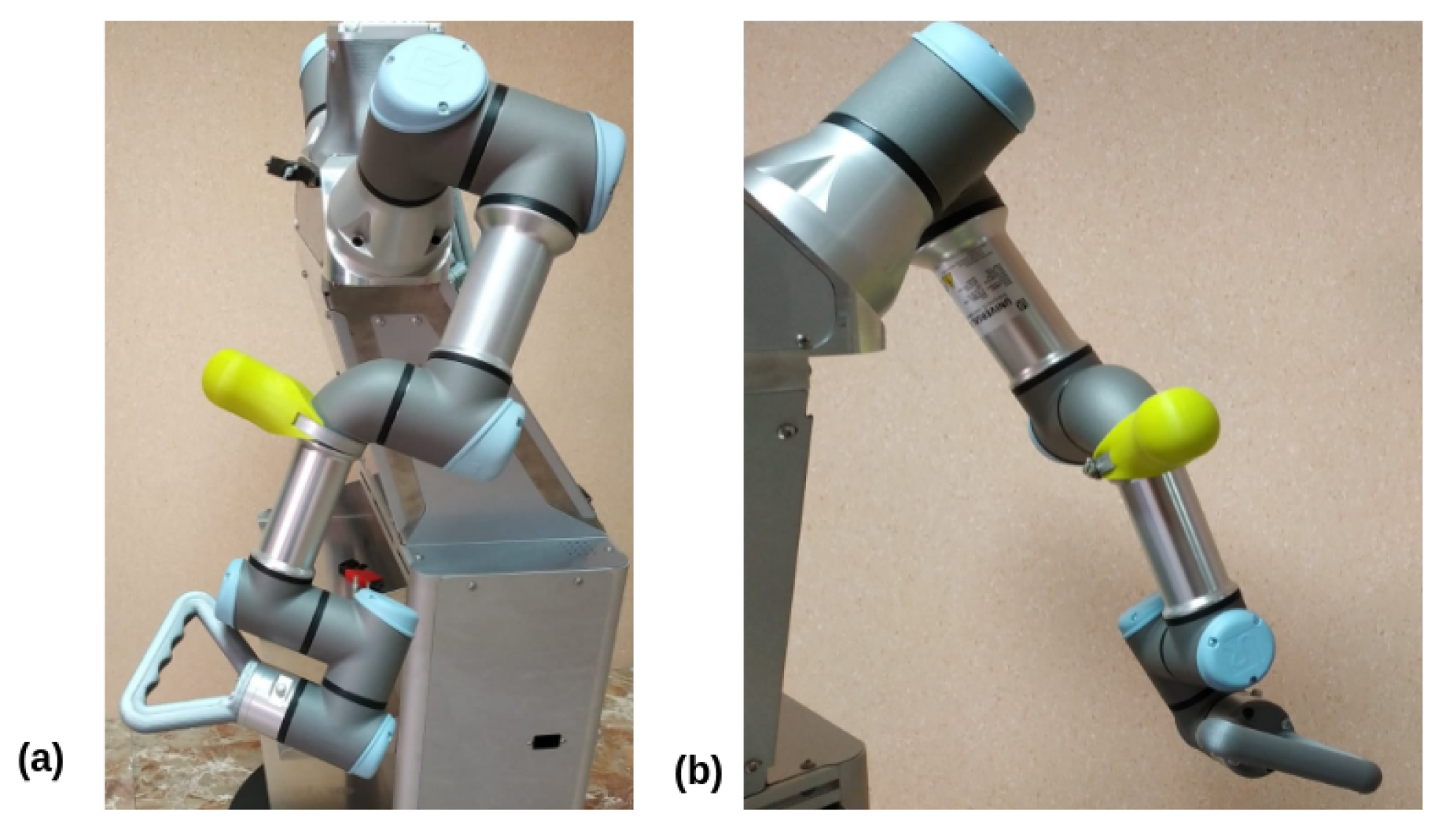
Table 1.
Characteristics of the different algorithms compared.
| Global Stability | Multiple Demonstrations | Single-Step Learning | Direct Application to Higher Dimension | |
|---|---|---|---|---|
| SEDS | Yes | Yes | No | No |
| CLF-DM | Yes | Yes | No | No |
| FSM-DM | Yes | Yes | No | No |
| UMIC | Yes | Yes | Yes | No |
| Modified DS | Yes | Yes | Yes | Yes |
| Out method (FML) | Yes | Yes | Yes | Yes |
Table 2.
Reproduction error of different methods on the LASA dataset.
| Method | Mean SEA (mm) | Mean (mm/s) |
|---|---|---|
| SEDS | 142.9 | |
| CLF-DM | 71.8 | |
| FSM-DM | 172.6 | |
| UMIC | 143.2 | |
| Modified DS | 56.9 | |
| Out method (FML) | 12.48 | |
| Out method (FML) | ||
| using auto-learning | − | 9.17 |
Disclaimer/Publisher’s Note: The statements, opinions and data contained in all publications are solely those of the individual author(s) and contributor(s) and not of MDPI and/or the editor(s). MDPI and/or the editor(s) disclaim responsibility for any injury to people or property resulting from any ideas, methods, instructions or products referred to in the content. |
© 2023 by the authors. Licensee MDPI, Basel, Switzerland. This article is an open access article distributed under the terms and conditions of the Creative Commons Attribution (CC BY) license (https://creativecommons.org/licenses/by/4.0/).
Share and Cite
MDPI and ACS Style
Prados, A.; Mora, A.; López, B.; Muñoz, J.; Garrido, S.; Barber, R. Kinesthetic Learning Based on Fast Marching Square Method for Manipulation. Appl. Sci. 2023, 13, 2028. https://doi.org/10.3390/app13042028
AMA Style
Prados A, Mora A, López B, Muñoz J, Garrido S, Barber R. Kinesthetic Learning Based on Fast Marching Square Method for Manipulation. Applied Sciences. 2023; 13(4):2028. https://doi.org/10.3390/app13042028
Chicago/Turabian StylePrados, Adrián, Alicia Mora, Blanca López, Javier Muñoz, Santiago Garrido, and Ramón Barber. 2023. "Kinesthetic Learning Based on Fast Marching Square Method for Manipulation" Applied Sciences 13, no. 4: 2028. https://doi.org/10.3390/app13042028
Note that from the first issue of 2016, this journal uses article numbers instead of page numbers. See further details here.