A Novel Two-Stage 3D-Printed Halbach Array-Based Device for Magneto-Mechanical Applications

Abstract

This research unveils a versatile Halbach array magnetic device with promising biomedical applications, offering innovative solutions for targeted therapy and disease management in evolving biomedical engineering. This paper explores the potential of a novel Halbach array-based device for harnessing magneto-mechanical phenomena in biomedical applications. The study employs computational modeling using COMSOL Multiphysics to define the device’s magnetic properties and validate its operation within the theoretical prediction. The research catalogs the device’s operational modes and assesses crucial parameters related to magneto-mechanical biomedical modalities, including magnetic field strength, gradient, and force. Experimental validation of numerical findings through magnetic field measurements confirms the device’s multifaceted potential, particularly in targeted drug delivery and tissue engineering applications. Finally, the adaptability of the magnetic arrangements for various scenarios is also highlighted. This investigation provides valuable insights into integrating magneto-mechanical principles into biomedical engineering. It paves the way for further research and innovative approaches in theranostics, positioning the presented apparatus as a promising tool with untapped potential for future exploration and discovery in the evolving biomedical field.

1. Introduction

The field of biomedicine has seen remarkable advancements in recent years, thanks to the rapid pace of technological progress and scientific creativity. One area of particular interest has been the development of new therapeutic applications, which continue to plague humanity despite decades of research. Magnetic fields have been used in biomedicine for various applications [1,2,3,4]. In diagnostics, Magnetic Resonance Imaging (MRI) is one of the most common applications of magnetic fields, providing detailed images of soft tissue and organs without the use of ionizing radiation [1,5,6,7]. In therapy, a technique that was heavily researched in recent years is Magnetic Particle Hyperthermia (MPH), which involves the use of magnetic nanoparticles to generate heat and destroy cancer cells [6,8,9]. Targeted drug delivery is another area where magnetic fields have shown great potential [10,11]. By attaching magnetic nanoparticles to drugs, it is possible to use magnetic fields to guide the particles to specific regions of the body, such as tumors or inflamed tissue. This approach allows for more precise drug delivery and reduced side effects [12,13].

In this context, researchers have turned to the principles of magneto-mechanics, that is, the exploitation of the magnetic energy of magnetic elements or chemical compounds by transformation into mechanical energy that manifests as forces and torques [14,15]. In general, magnetic fields significantly weaker than one tesla strength are utilized. For alternating magnetic fields (AMFs), the range of optimal frequencies falls under the Extremely Low Frequency (ELF) range (f < 100 Hz), since in higher magnitudes, the thermal effects become dominant (in the first approximation, heating is directly proportional to the frequency of the field) [16,17]. In the biomedical field, this definition is further constrained by the size of the particles that are required to be lower than the microscale.

Among magneto-mechanical approaches, Halbach arrays have gained prominence [18,19,20]. This magnet arrangement, characterized by alternating polarities of neighboring magnets, creates strong localized magnetic fields through constructive and destructive interference. Originating in the 1980s [21], Halbach arrays have found applications in diverse fields, from particle accelerators to magnetic levitation trains [22]. Their potential in biomedicine stems from the ability to generate highly localized magnetic fields and gradients with minimal energy loss [23,24,25].

This paper delves into the design, manufacturing, simulation, and experimental validation of a custom multimodal magnetic field generator featuring two circular and rotating Halbach arrays. Calculations of magnetic flux density and corresponding magnetic forces on nanoparticles of varying sizes are presented for static and time-dependent scenarios. The study investigates the impact of the vertical distance between the arrays in the static case and explores the temporal distribution of magnetic field gradients during rotation. The synergy of field and gradient configurations, in conjunction with magnetically suitable nanoparticles, is demonstrated to produce a spectrum of forces with potential biological effects. The versatility of this device, coupled with its comprehensive field and force roadmaps, positions it as a valuable reference apparatus for future investigations into magneto-mechanical effects on cellular environments.

2. Materials and Methods

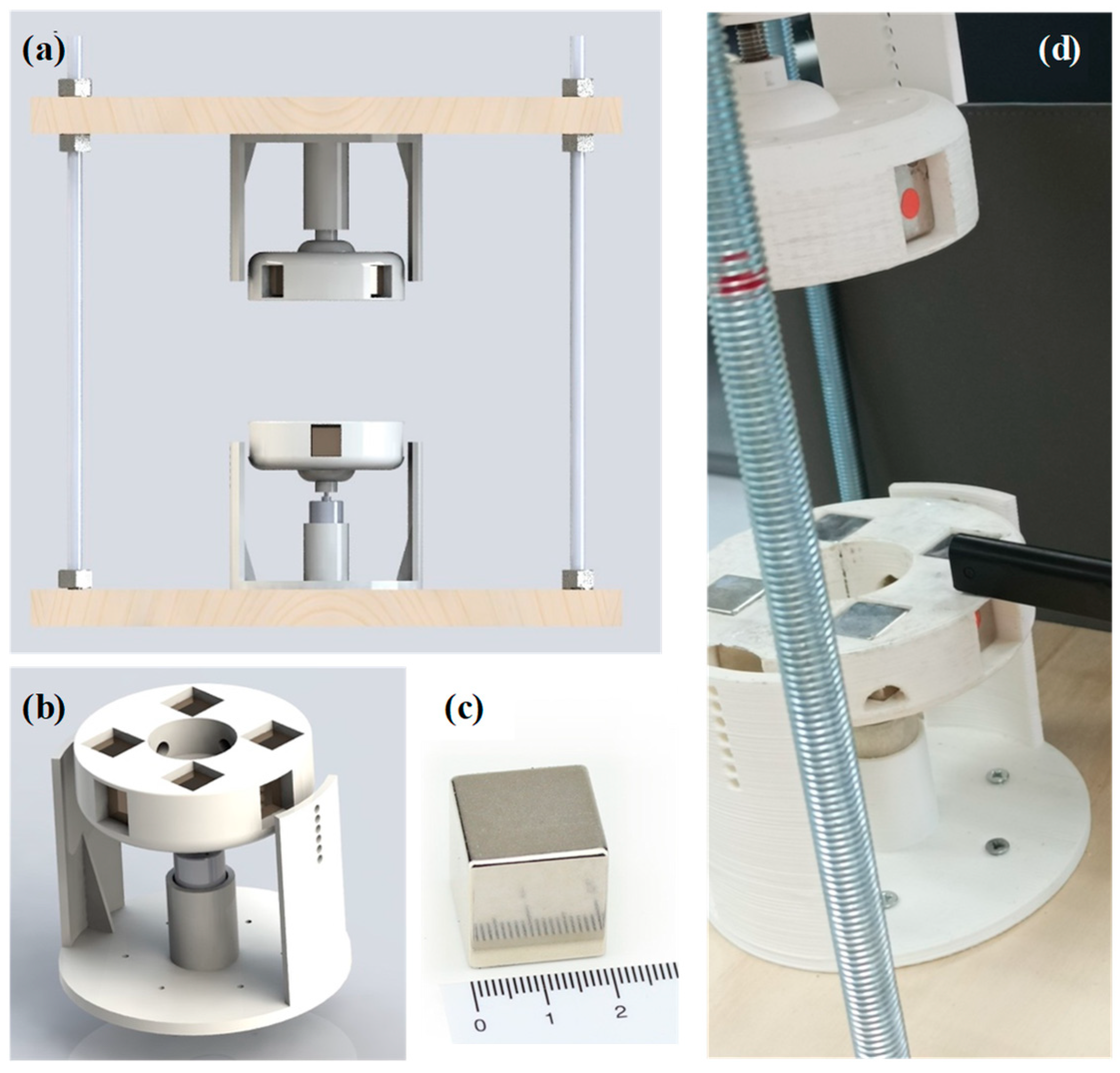
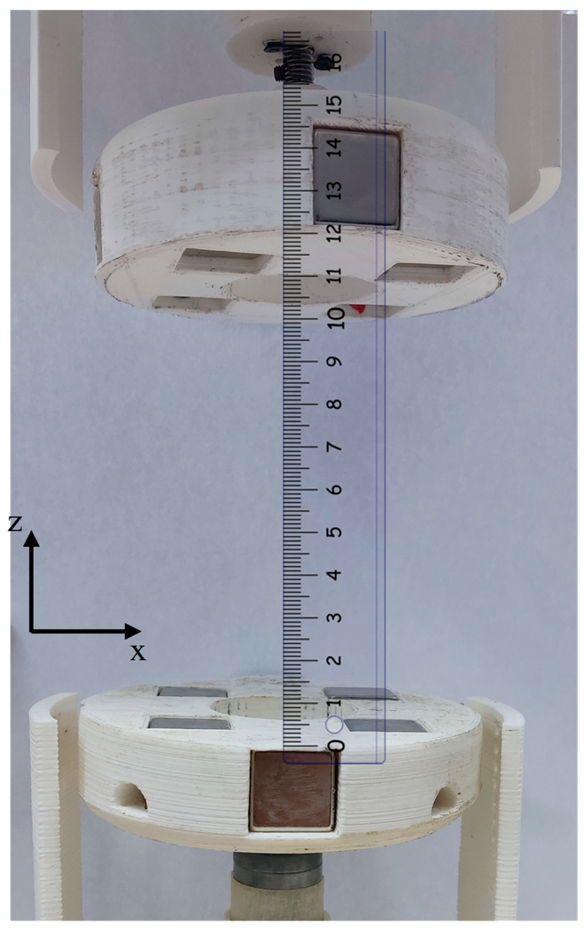
2.1. Experimental Apparatus (Design/Manufacture)

The proposed setup that utilizes two circular Halbach arrays is presented in Figure 1. The second array is of identical radius and is positioned along the vertical axis that intercepts the center of the xy plane that the first array defines, forming a normal angle. To hold the arrays in place, two 3D-printed disks are utilized. The choice of this geometry, that is, the positioning of a second array vertically above the first one, is based on our previous works [26,27], where the analysis of a single disk apparatus resulted in the generation of strong gradients and simultaneously large magnetic flux densities, optimizing the magneto-mechanical effect on cell actuation. The proposed experimental geometry is illustrated in Figure 1.

The disks as well as their mounts, were designed in AutoCAD Inventor and were proceeded to be 3D-printed using a simple polymer. The disks were designed to host cubic permanent magnets and a motor that can rotate each array with a constant angular velocity. Two legs were printed on either side of the disk with nooks at equal distances and near the height of the disk. Those alcoves are utilized to mount a bracket-shaped table on top of which a typical petri dish (3.5 cm) can be placed for in vitro testing (Figure 1b). The printed disks are screwed on two flush wood planks that are subsequently connected with four screw rods, in a manner that makes each disk the mirror of the other. The top wooden platform is secured with bolt nuts in both directions allowing for an adjustable distance between the disks (Figure 1a). In the experiments, the distance of the disks is set to 10.3 cm. Each disk can host a total of eight cubic magnets arranged in a way that every magnet is equidistant (5 mm) to its neighboring magnets and that the inner side of the magnets inserted by the side of the disk is 2.5 cm away from the center. Finally, a circle-shaped hole, with a radius of 2 cm, that goes as deep as the magnets’ height, is created in the center to offer a wider range of z-levels in the single disk setup.

The magnets (Figure 1c) placed in the 2 × 2 × 2 cm³ slots are permanent NdFeB N45 magnets sold commercially by EarthMag GmbH (Dortmund, Germany). The cubes have a remanent magnetic flux density B_r = 1.33–1.36 T and a relative magnetic permeability μ_r = 1.05 due to them being made of NdFeB.

The motors operate on DC and their frequency of rotation can be adjusted by inputting a different voltage. More specifically, a range of 3–12 volts is operational, resulting in a range of 0–12 Hz in rotational motion. In this work, the motors rotate the arrays with a frequency of 6.67 Hz.

2.2. Computational Modelling (Simulation)

Calculating the theoretical values of the magnetic field in the space between the two disks is an arduous time-consuming venture, if attempted to be done, even with the aid of computing power. An easier approach is to code the problem at hand into a Finite Element Analysis-based software. COMSOL v. 3.5a Multiphysics belongs in this category with the advantage of having physics libraries that can completely describe the phenomena taking place in this setup. In order to successfully emulate the behavior of the setup, the magnetic as well as the mechanical properties of the apparatus need to be described.

The library that is used to simulate the generated magnetic field solves the differential equation [28] of the scalar magnetic potential V_m:

$$-\overrightarrow{\nabla }·\left({\mu }_0{\mu }_r\overrightarrow{\nabla }{V}_m-{\overrightarrow{B}}_r\right)=0$$

(1)

where B_r is the remanent magnetic field and μ_r is the relative magnetic permeability. Depending on the subdomain described, the parameters of the equation are assigned the appropriate values that correspond to the magnetic characteristics of the permanent magnets or their surrounding environment. The magnetic field strength at a given point of the simulated area is, thus, given by the equation

$$\overrightarrow{B}={\mu }_0{\mu }_r{\overrightarrow{H}}_a+{\overrightarrow{B}}_r$$

(2)

Besides the applied magnetic field intensity H_α, which is defined by the solution of (1), the parameters of (2) are set as subdomain conditions manually.

A cylinder surrounding the magnet compositions is set as the boundary of magnetic insulation; this reduces the computing power required to solve the problem. In other words, the cylinder contains the condition

$$\overrightarrow{n}·\overrightarrow{B}=0$$

(3)

The intersurface between the NdFeB magnets and the environment in the large cylinder is set with a continuity boundary condition. The condition is expressed by the following equation:

$$\overrightarrow{n}·\left({\overrightarrow{B}}_1-{\overrightarrow{B}}_2\right)=0$$

(4)

where B₁ and B₂ are the magnetic flux densities inside and outside the intersurface.

For the mechanical rotation of the circular arrays, the finite elements that fill the area of the boundary cylinder are rotated around the z-axis. This procedure is equivalent to the physical rotation of the drawn objects, due to the fact that each dividend contains the magnetic field conditions of its coordinates that are true for the apparatus in a static state. The mechanical movement of each element is expressed by defining the time-dependent coordinates:

$$\begin{array}{c}dz=0\\ dx=\cos \left(-\omega t\right)·X-\sin \left(-\omega t\right)·Y-X\\ dy=\sin \left(-\omega t\right)·X+\cos \left(-\omega t\right)·Y-Y\end{array}$$

(5)

where X and Y are the values of each element prior to the rotation ($t=0$), ω is the angular velocity that is described in the motors’ specifications. This set of Equation (5) describes a clockwise rotation with constant angular velocity.

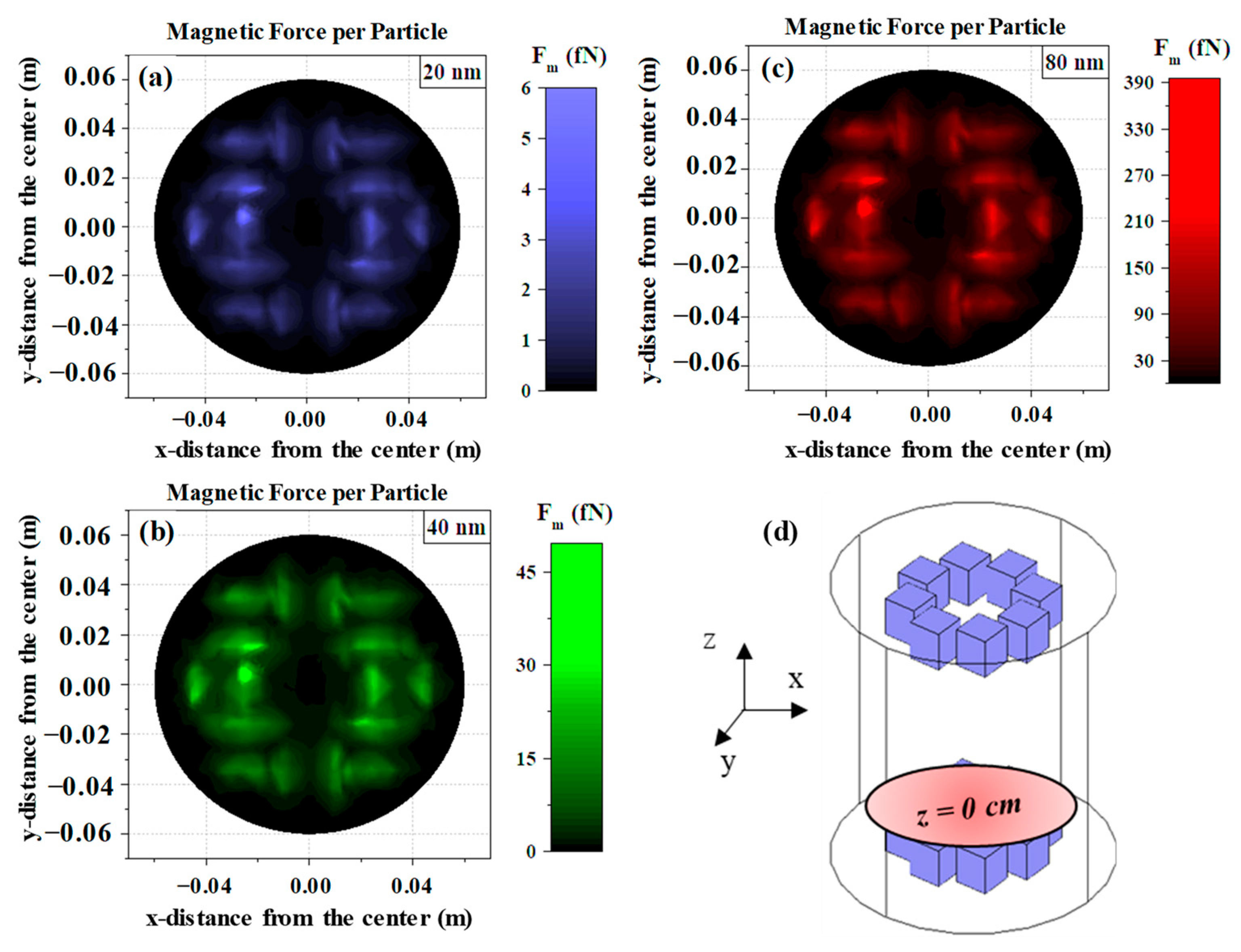
2.3. Force Estimation

Although the simulation of the magnetic strength and gradient is a straightforward task requiring basic calculus knowledge, the process of modelling the magnetic forces is more complicated. This is due to the plethora of interactions at play between particles and the environment that they are suspended in. By assuming the magnetic forces to be significantly greater than the other interactions, hence rendering the latter negligible, a model was developed by Furlani et al. [29] that has been used in most modelling works in the recent literature [26,30].

For the linear magnetization of perfectly spherical particles, Equations (6) and (7), respectively, are true:

$$\overrightarrow{M}={\chi }_p{\overrightarrow{H}}_{in}$$

(6)

$${\overrightarrow{H}}_d=\frac{\overrightarrow{M}}{3}$$

(7)

where ${\chi }_p$ is the magnetic susceptibility of the particles, while the demagnetizing intensity ${\overrightarrow{H}}_d$ and the magnetic field inside the particle ${\overrightarrow{H}}_{in}$ are connected by the expression

$${\overrightarrow{H}}_{in}={\overrightarrow{H}}_a-{\overrightarrow{H}}_d$$

(8)

Combining Equations (6)–(8), the magnetization vector can be expressed as

$$\overrightarrow{M}=\frac{3{\chi }_p}{3+{\chi }_p}{\overrightarrow{H}}_a$$

(9)

From here, the magnetic force exerted by one particle after some thorough analysis is proven to be given by the expression

$${\overrightarrow{F}}_{mp}={\mu }_0{V}_p\frac{3{\chi }_p}{3+{\chi }_p}\left({\overrightarrow{H}}_a·\overrightarrow{\nabla }\right){\overrightarrow{H}}_a$$

(10)

where $V_p=\frac{4}{3}\pi r_p^3$ is the volume of a spherical particle with $r_p$ the radius of the particle.

Equation (10) can be split into three one-dimensional equations along the axes of a cartesian coordinate system for each one of ${\overrightarrow{F}}_{mp}$ constituents:

$$\begin{array}{c}{F_i}_{mp}^x={\mu }_0{V}_p\frac{3{\chi }_p}{3+{\chi }_p}\left[\begin{array}{c}{H}_a^x\left(x,y,z\right)\frac{\partial H_a^x}{\partial x}\\ H_{\alpha }^y\left(x,y,z\right)\frac{\partial H_a^x}{\partial y}\\ H_a^z\left(x,y,z\right)\frac{\partial H_a^x}{\partial z}\end{array}\right]\\ {F_i}_{mp}^y={\mu }_0{V}_p\frac{3{\chi }_p}{3+{\chi }_p}\left[\begin{array}{c}{H}_a^x\left(x,y,z\right)\frac{\partial H_{\alpha }^y}{\partial x}\\ H_{\alpha }^y\left(x,y,z\right)\frac{\partial H_{\alpha }^y}{\partial y}\\ H_a^z\left(x,y,z\right)\frac{\partial H_{\alpha }^y}{\partial z}\end{array}\right]\\ {F_i}_{mp}^z={\mu }_0{V}_p\frac{3{\chi }_p}{3+{\chi }_p}\left[\begin{array}{c}{H}_a^x\left(x,y,z\right)\frac{\partial H_a^z}{\partial x}\\ H_{\alpha }^y\left(x,y,z\right)\frac{\partial H_a^z}{\partial y}\\ H_a^z\left(x,y,z\right)\frac{\partial H_a^z}{\partial z}\end{array}\right]\end{array}$$

(11)

where the terms in the equations set (11) are the x, y and z components of the vectors ${\overrightarrow{F}}_{mp}\mathrm{and}{\overrightarrow{H}}_a.$ The magnetic force evaluation is conducted with particles that exhibit ferromagnetic behavior in mind. Thus, the fraction $3{\chi }_p/\left(3+{\chi }_p\right)$ in (11) can be replaced by a scalar factor equal to three, since for ferromagnetic particles, ${\chi }_p\gg 1$. These are the equations that are used in the COMSOL simulation to emulate the exerted magnetic forces per particle. To consider the total force applied to an ensemble of N particles, (non-interacting or negligibly interacting) the equation below is utilized:

$${\overrightarrow{F}}_{tot}={\displaystyle \sum }_{i=1}^N{{\overrightarrow{F}}_i}_{mp}$$

(12)

2.4. Computational Steps

To obtain results, we employed the following computational steps:

Model Navigator: On the New page in the Model Navigator of COMSOL Multiphysics, we specified the application mode which was the AC/DC mode with a moving mesh, the names of the dependent variables, and the analysis type, which was the transient (time-dependent) analysis with a time step that was equal to 0.01 s.

Options and Settings: We set the axes and grid spacing. All settings were accessible from the Options menu. We also used the Constants dialog box to enter constant parameters for the model. The materials used were accessible through the Materials/Coefficients Library dialog of COMSOL Multiphysics. From the Options menu, by choosing “Expressions → Global Expressions”, we imported the Equations (6)–(10) as expressions for the analytical solution of the magnetic force.

Geometry Modeling: We imported the device geometry that was designed in AutoCAD Inventor.

Boundary Conditions: An important technique to minimize the problem size is to use the magnetic insulation boundary condition at the outer boundaries of the model geometry. In the inner boundaries of the geometry, we employed the continuity boundary condition. This is the natural boundary condition implying continuity of the tangential component of the magnetic field.

Subdomain Settings: We then defined the subdomain parameters of the physical problems with regions of different material properties. Some of the domain parameters can either be a scalar or a matrix depending on if the material is isotropic or anisotropic.

Scalar Variables: In the Application Scalar Variables dialog box, we examined and modified the values of predefined application-specific scalar variables. These were the frequency of rotation and the permittivity and permeability of vacuum.

Mesh Generation: The program must mesh the geometry before it can solve the problem. The mesh consisted of 3 × 10⁶ elements and 20 degrees of freedoms (DOFs) per mesh element.

Computing the Solution: We used the Geometric multigrid (GMG) preconditioner as an iterative linear solver. The solver calculates the solution for the finest of the meshes in the hierarchy. Therefore, we let the preconditioner generate the meshes automatically and we obtained a solution for a much finer mesh than the one we had made.

Postprocessing and Visualization: After solving the problem, the software automatically displays a surface plot for the dependent variables, in this case, the magnetic vector potential and the magnetic flux density. Magnetic gradient and force distribution can also be obtained by calling the corresponding function that was user-defined in step 2.

3. Results and Discussion

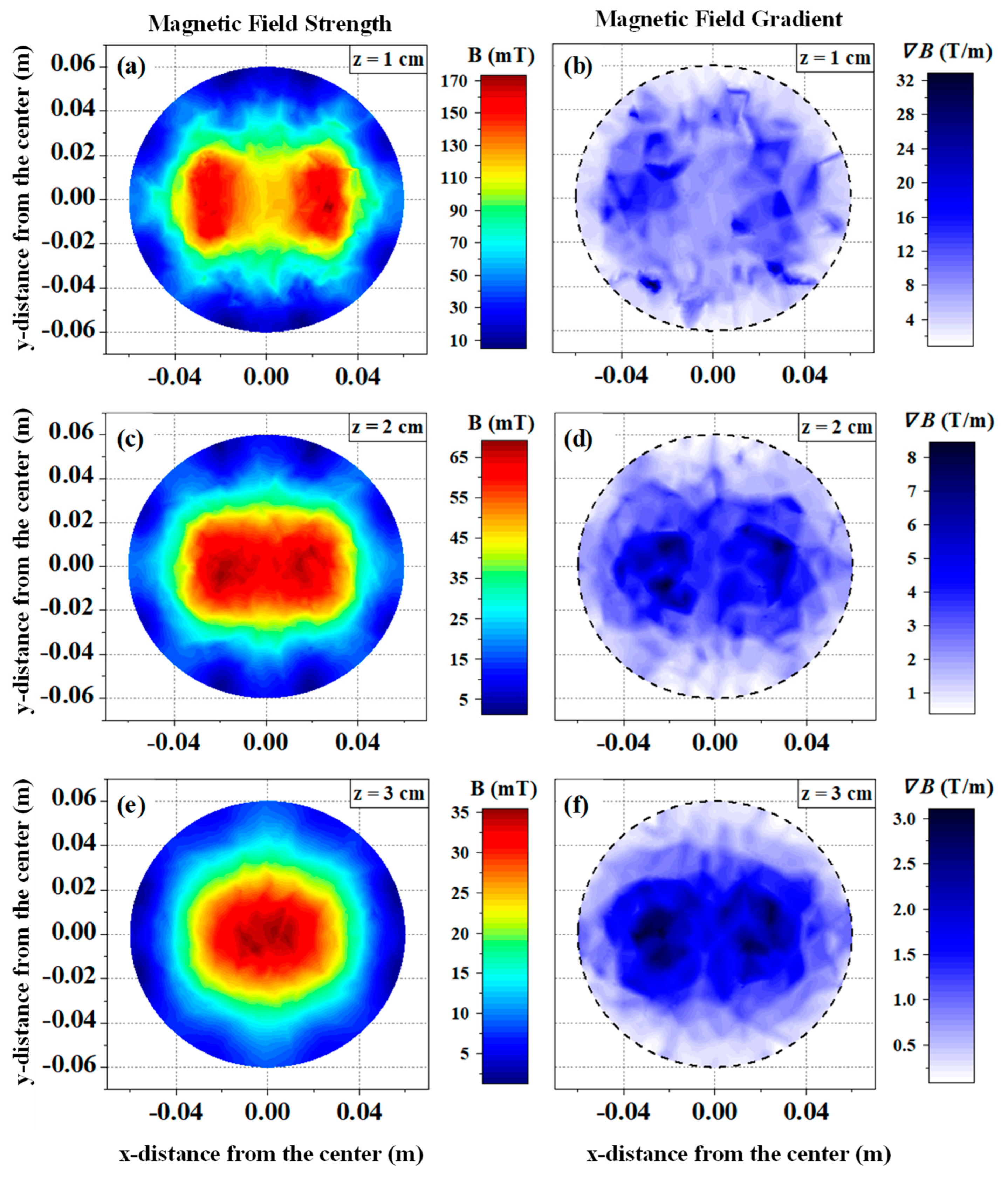
Keeping in mind the nature of the biological assays that can be conducted with the proposed setup, it is beneficial to visualize the computational data onto slice plots, normal to the z-axis.

3.1. Static Study

The data corresponding to the static scenario are illustrated utilizing contour plots, where the axes correspond to the x and y coordinates and the color contouring is used to express the varying magnitude of the magnetic flux density, its gradient, or the exerted magnetic forces. Indicatively, slice plots of the latter in distances near the bottom array are presented in the following figures. Figure 2 gives a schematic illustration of the two disks and the z-levels that will be presented in the following sections.

In Figure 3, slice plots of the magnetic flux density and its gradient at varying distances (1, 2, and 3 cm) above the bottom Halbach array are presented. Based on the morphology of the graphs, a convergence of the homogeneity area (with the strongest magnetic field) towards the center, as the distance from the disks increases, is observed. The registered planes show the existence of three homogenous areas that can be found at the center of each magnet configuration and at the plane that is equidistant to both Halbach arrays. This phenomenon further extends the range of applications, due to the variation in the “red surface” area providing with larger magnetic gradients to cell cultures and/or animals if positioned properly.

The exerted forces per ferromagnetic particle of varying size (20, 40, and 80 nm in diameter, core size) are illustrated as contour plots. Here, the maximal values are presented, which correspond to a 2 mm distance from one or the other array. Pointedly, Figure 4 depicts the slice plots above the bottom array. Considering the force range per particle, a biomedical assessment will follow based on force thresholds of biomedical functions that are of interest in relevant applications.

The results depicted in Figure 3 and Figure 4 concern the setup with both Halbach arrays generating the magnetic field. Due to the adjustability of the apparatus, a singular disk configuration can be utilized. Its magnetic properties were explored using COMSOL and the numerical analysis results are illustrated in Figure S1.

The process of gauging the setup’s capabilities for biomedical applications is concluded with a comparison of the force thresholds for mechano-sensitive cellular functions and for integrity compromise. Such thresholds have been registered in the literature [16,31] and are collected in Figure 5, together with the minimum (for single particle only) and maximum (assembly of 1000 particle) force value achieved by the proposed device, depicted by the magenta zone in Figure 5. Force estimations were completed for a system of 20 nm magnetite nanoparticles. A recently published paper by Tran and Matsushita [32] highlights the magnetic behavior of L10 FePt nanoparticles as their size decreases, transitioning to superparamagnetic behavior wherein thermal fluctuations become comparable to the energy barrier for magnetic flips. It is important to mention here that lower-sized nanoparticles (less than 20 nm) may exhibit superparamagnetic behavior at room temperature. Consequently, the total force applied by our system will be significantly weaker for such nanoparticles. On the other hand, A. Moghanizadeh et al. [33] demonstrated that increasing the intensity of the magnetic field from 0.1 to 0.3 T led to a substantial increase in the clot dissolution rate from 55 to 89%, respectively. Remarkably, this magnetic field range aligns with the capabilities of our device, suggesting potential applicability in thrombolysis and other biomedical interventions. These findings underscore the versatility and effectiveness of magnetic field-mediated therapies, further supporting the potential utility of our device across a range of biomedical applications. In addition, our device’s capability to create a total homogeneous magnetic field with a Halbach array, while also providing high magnetic field gradients, offers unprecedented opportunities for advancing the applications discussed previously by A. Sandhu and H. Handa [34]. By integrating insights from the aforementioned book with the capabilities of our device, we envision transformative advancements in medical diagnostics, enhancing sensitivity, accuracy, and efficiency in healthcare.

From the threshold values presented Figure 5, it becomes evident that for an ensemble of 10³ magnetite nanoparticles, functions and operations requiring forces of the order of 100 pN can easily be activated/initiated as the generated forces for this hypothetical scenario are well over that value. Generating forces in the order of nN, however, would require a larger concentration of Magnetic Nanoparticles (MNPs) in the targeted site or, alternatively, nanoparticles of a bigger size. Surprisingly, unlike the literature where particles larger than 100 nm have been proven to be more suitable for magneto-mechanical cell actuation [27], with the proposed apparatus, even smaller particles of 20 nm can magneto-mechanically trigger the cells’ biological effects.

3.2. Rotational Study

Following the numerical analysis of the static case study, a similar approach is followed to highlight the ability of the setup for generating time-dependent magnetic field modes. In this paper, the Alternating Magnetic Field (AMF) mode is explored. Contrary to the previous simulation results, in this scenario, a dual axis format is used for two characteristic points in every xy parallel plane between the arrays. These points have the coordinates (0, 0, z) and (3, 0, z) (units are in cm) and are denoted as C and R, respectively. Figure 6a–d illustrates the functions B(t) and ∇B(t). The simulations are conducted for one revolution, at varying distances (z-levels), as shown in Figure 6e between the disks.

In Figure 7, the maximal magnetic force amplitudes are presented. Following the same color coding as in Figure 6, the three sizes of ferromagnetic particles are analyzed numerically for the plane that is only two millimeters above the bottom array (z = 2.2 cm).

Considering the curves shown below, it is deduced that the setup can, in theory, produce harmonic AMFs with an adjustable frequency that can be tuned by the voltage applied to the motors. It is important to note that, on the periphery of the conceived cylinder, the data have a sinusoidal form, but because of the logarithmic scale, they are deformed in the following figures. Additionally, the homogeneity subdomain is demonstrated by the infinitesimal peak-to-peak magnetic field amplitude of the quantities at the center of plane C, as shown in Figure 7b.

In Figure S2, a larger collection of generated time-dependent forces for the three sizes of MNPs can be found at different distances from the arrays.

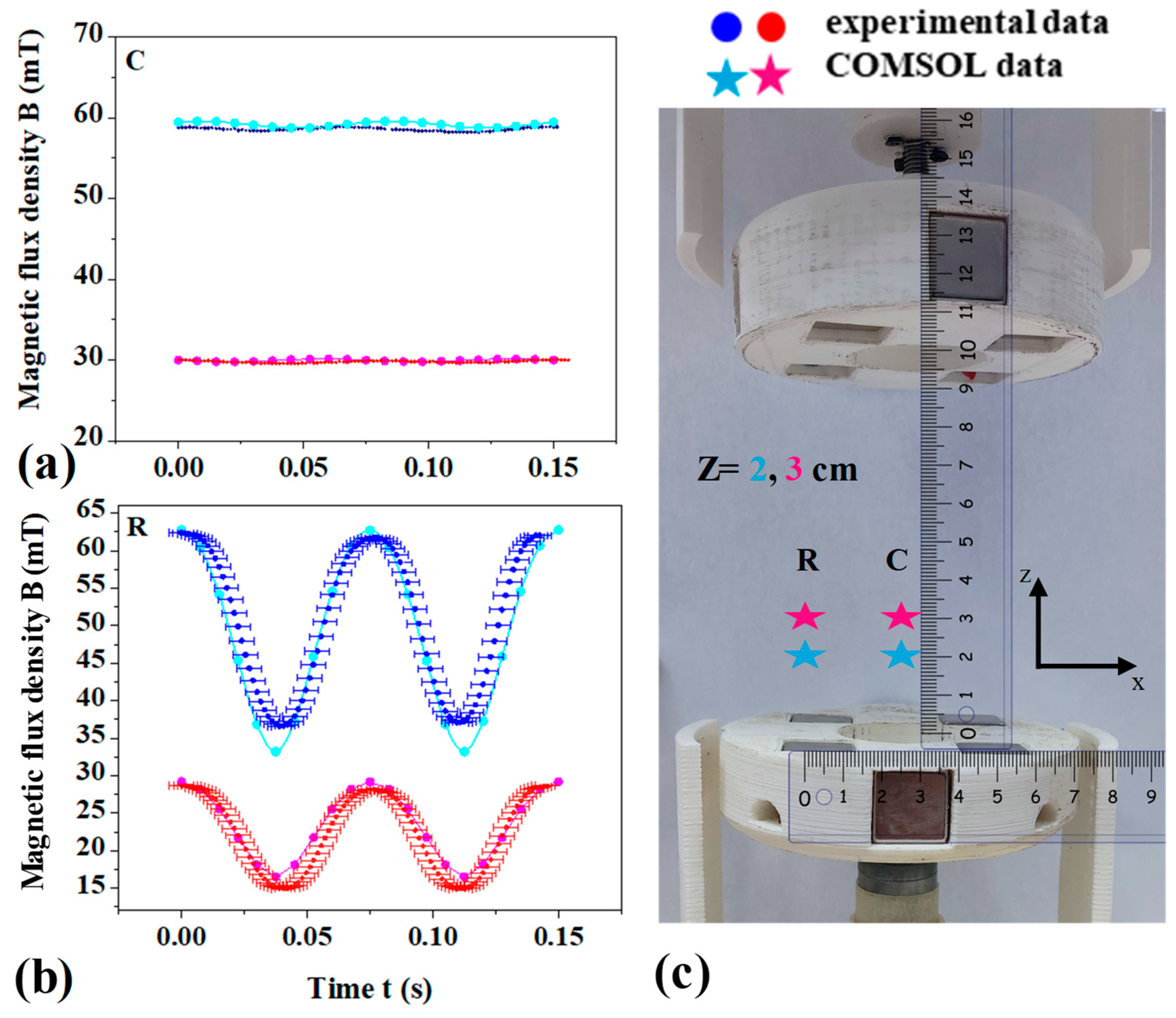
3.3. Experimental Validation

The experimental validation of the computationally derived magnetic flux density B is executed with the aid of Metrolab’s three-axis magnetometer, THM1176-MF model (Figure 8) that offers a range of 100 mT extending up to 3 T. The instrument has an accuracy of ±1% of the value read, or 0.1 mT depending on which one is of larger magnitude. For a frequency of rotation around 6.67 Hz, the magnetometer provides more than sufficient “time resolution” given that its acquisition rate can comfortably capture 100 points per period (≈0.15 s).

The magnetometer is placed strategically in different positions in the xy planes, the choice of which is influenced by the spatial resolution of the instrument to avoid measurement overlapping.

When evaluating the static behavior of the apparatus, an average of 7% deviation from the numerical analysis results was recorded. Indicatively, in Figure 9, a visualization of the experimental data in front of a slice plot, one cm away from the bottom array is provided. The dataset’s size is defined by the spatial resolution of the instrument. The latter additionally restricts the measurements of the field, rendering it safer to collect data further away from the arrays.

Similarly, for the assessment of the rotational mode, the Hall probe measures the magnetic flux density at C (0, 0, z) and R (3, 0, z) with units in cm, while the arrays are rotating with a constant angular velocity. In Figure 9, the experimental data for z = 2 and z = 3 cm are illustrated, along with the corresponding curves that the computational model predicts. The convergence of the numerical analysis results with the Hall probe measurements is evident. It is also important to mention here that the non-magnetic nature of the outer metal components, excluding the magnets themselves, ensures minimal interference with the precise measurement of the total magnetic field mapping, as corroborated by Hall probe measurements.

The great convergence of the experimental data with the numerical analysis results, both in the static and the rotating disks mode, ensures that the model can be safely utilized to identify the ideal subdomain for any biomedical assay.

The strong agreement between the experimental data and numerical analysis results, observed in both static and rotating disk modes, validates the reliability of our model. This validation assures its suitability for accurately identifying the optimal subdomain for various biomedical assays.

4. Conclusions

This paper has explored a novel setup of Halbach arrays that was designed to harness the magneto-mechanical effect in biomedicine. The apparatus’ versatility was demonstrated by inspecting two of the possible magnetic field modes. Using COMSOL 3.5a Multiphysics, the magnetic characteristics of the generated field, spatially and temporally, were derived through a numerical analysis. The outcomes of this study highlighted the setup’s capabilities for achieving the necessary conditions for the magneto-mechanical effect to manifest. The analysis was subsequently extended to a calculation of the magnetic force exerted by a spherical particle when exposed to the described magnetic conditions following an effective dipole approximation. Our computational findings for three scenarios of ferromagnetic magnetite nanoparticles suggested the generation of forces up to hundreds of pN when an ensemble of 10³ MNPs successfully reaches the targeted site. Comparing the order of forces to various cellular functions and tensile strengths, we concluded the overcoming of said thresholds, rendering the device a more than capable tool to mediate magneto-mechanical effects that are investigated for biomedical applications in recent times. At last, the numerical analysis was confirmed by experimental measurements using a Hall magnetometer for a static and rotational study. The results proved the device’s reliability, showing a great convergence with the computational model.

Although mitigating interactions between the particles and the environment (e.g., drag forces when the particles are suspended in a fluid) have not been accounted for here, previous in vitro studies conducted in our laboratory with a similar 3D-printed setup have yielded successfully selective apoptosis and cell deformation among other effects. Given that this setup utilizes the Halbach configuration, an improvement compared to its predecessor, dominant opposing forces, cannot typically negate the generated forces to a point where the threshold at hand is not surpassed.

Significantly, this work opens up a vast range of applications from magneto-genetics to cancer therapy. Having demonstrated its reliability and potency, future research entails assays with biological samples both in vitro and in vivo to attest our findings and to further advance the magneto-mechanical approach in biomedicine.

References

1. Barinec, P.; Krafčík, A.; Babincová, M.; Rosenecker, J. Dynamics of magnetic particles in cylindrical Halbach array: Implications for magnetic cell separation and drug targeting. Med. Biol. Eng. Comput. 2010, 48, 745–753. [Google Scholar] [CrossRef] [PubMed]
2. Pankhurst, Q.A.; Thanh NT, K.; Jones, S.K.; Dobson, J. Progress in applications of magnetic nanoparticles in biomedicine. J. Phys. D Appl. Phys. 2009, 42, 224001. [Google Scholar] [CrossRef]
3. Berry, C.C.; Curtis, A.S.G. Functionalisation of magnetic nanoparticles for applications in biomedicine. J. Phys. D Appl. Phys. 2003, 36, R198. [Google Scholar] [CrossRef]
4. Makridis, A.; Kazeli, K.; Kyriazopoulos, P.; Maniotis, N.; Samaras, T.; Angelakeris, M. An accurate standardization protocol for heating efficiency determination of 3D printed magnetic bone scaffolds. J. Phys. D Appl. Phys. 2022, 55, 435002. [Google Scholar] [CrossRef]
5. Vergallo, C.; Ahmadi, M.; Mobasheri, H.; Dini, L. Impact of inhomogeneous static magnetic field (31.7–232.0 mT) exposure on human neuroblastoma SH-SY5Y cells during cisplatin administration. PLoS ONE 2014, 9, e113530. [Google Scholar] [CrossRef] [PubMed]
6. Brown, M.A.; Semelka, R.C. MRI: Basic Principles and Applications; Wiley-Liss: New York, NY, USA, 1999. [Google Scholar]
7. Tao, C.; Chen, Y.; Wang, D.; Cai, Y.; Zheng, Q.; An, L.; Lin, J.; Tian, Q.; Yang, S. Macromolecules with Different Charges, Lengths, and Coordination Groups for the Coprecipitation Synthesis of Magnetic Iron Oxide Nanoparticles as T 1 MRI Contrast Agents. Nanomaterials 2019, 9, 699. [Google Scholar] [CrossRef] [PubMed]
8. Makridis, A.; Okkalidis, N.; Trygoniaris, D.; Kazeli, K.; Angelakeris, M. Composite magnetic 3D-printing filament fabrication protocol opens new perspectives in magnetic hyperthermia. J. Phys. D Appl. Phys. 2023, 56, 285002. [Google Scholar] [CrossRef]
9. Phadatare Manisha, R.; Meshram, J.V.; Gurav, K.V.; Kim, J.H.; Pawar, S.H. Enhancement of specific absorption rate by exchange coupling of the core–shell structure of magnetic nanoparticles for magnetic hyperthermia. J. Phys. D Appl. Phys. 2016, 49, 095004. [Google Scholar] [CrossRef]
10. Kianfar, E. Magnetic nanoparticles in targeted drug delivery: A review. J. Supercond. Nov. Magn. 2021, 34, 1709–1735. [Google Scholar] [CrossRef]
11. Kharat, P.B.; Somvanshi, S.B.; Jadhav, K.M. Multifunctional magnetic nano-platforms for advanced biomedical applications: A brief review. J. Phys. Conf. Ser. 2020, 1644, 012036. [Google Scholar] [CrossRef]
12. Mitchell, M.J.; Billingsley, M.M.; Haley, R.M.; Wechsler, M.E.; Peppas, N.A.; Langer, R. Engineering precision nanoparticles for drug delivery. Nat. Rev. Drug Discov. 2021, 20, 101–124. [Google Scholar] [CrossRef] [PubMed]
13. Angelakeris, M. Magnetic nanoparticles: A multifunctional vehicle for modern theranostics. Biochim. Biophys. Acta BBA 2017, 1861, 1642–1651. [Google Scholar] [CrossRef]
14. Nikitin, A.A.; Ivanova, A.V.; Semkina, A.S.; Lazareva, P.A.; Abakumov, M.A. Magneto-mechanical approach in biomedicine: Benefits, challenges, and future perspectives. Int. J. Mol. Sci. 2022, 23, 11134. [Google Scholar] [CrossRef] [PubMed]
15. Hu, B.; El Haj, A.J.; Dobson, J. Receptor-targeted, magneto-mechanical stimulation of osteogenic differentiation of human bone marrow-derived mesenchymal stem cells. Int. J. Mol. Sci. 2013, 14, 19276–19293. [Google Scholar] [CrossRef] [PubMed]
16. Golovin, Y.I.; Gribanovsky, S.L.; Golovin, D.Y.; Klyachko, N.L.; Majouga, A.G.; Master, A.M.; Sokolsky, M.; Kabanov, A.V. Towards nanomedicines of the future: Remote magneto-mechanical actuation of nanomedicines by alternating magnetic fields. J. Control. Release 2015, 219, 43–60. [Google Scholar] [CrossRef]
17. Veselov, M.M.; Uporov, I.V.; Efremova, M.V.; Le-Deygen, I.M.; Prusov, A.N.; Shchetinin, I.V.; Savchenko, A.G.; Golovin, Y.I.; Kabanov, A.V.; Klyachko, N.L. Modulation of α-Chymotrypsin Conjugated to Magnetic Nanoparticles by the Non-Heating Low-Frequency Magnetic Field: Molecular Dynamics, Reaction Kinetics, and Spectroscopy Analysis. ACS Omega 2022, 7, 20644–20655. [Google Scholar]
18. Thalmayer, A.S.; Zeising, S.; Fischer, G.; Kirchner, J. Steering magnetic nanoparticles by utilizing an adjustable linear Halbach array. In Proceedings of the 2021 Kleinheubach Conference, Miltengerg, Germany, 28–30 September 2021; pp. 1–4. [Google Scholar]
19. Rana, S.M.S.; Salauddin, M.; Sharifuzzaman; Lee, S.H.; Shin, Y.D.; Song, H.; Jeong, S.H.; Bhatta, T.; Shrestha, K.; Park, J.Y. Ultrahigh-Output Triboelectric and Electromagnetic Hybrid Generator for Self-Powered Smart Electronics and Biomedical Applications. Adv. Energy Mater. 2022, 12, 2202238. [Google Scholar] [CrossRef]
20. Gibson, G.; Hailing, F.U. Wireless Power Transfer Using A Halbach Array and A Magnetically Plucked Piezoelectric Transducer for Medical Implants. In Proceedings of the 21st International Conference on Micro and Nanotechnology for Power Generation and Energy Conversion Applications (PowerMEMS), Salt Lake City, UT, USA, 12–15 December 2022; pp. 50–53. [Google Scholar]
21. Halbach, K. Design of permanent multipole magnets with oriented rare earth cobalt material. Nucl. Instrum. Methods 1980, 169, 3605–3608. [Google Scholar] [CrossRef]
22. Post, R.F.; Ryutov, D.D. The inductrack: A simpler approach to magnetic levitation. IEEE Trans. Appl. Supercond. 2000, 10, 901–904. [Google Scholar] [CrossRef]
23. Fuwa, Y.; Takayanagi, T.; Iwashita, Y. Development of Combined-Function Multipole Permanent Magnet for High-Intensity Beam Transportation. IEEE Trans. Appl. Supercond. 2022, 32, 4006705. [Google Scholar] [CrossRef]
24. Xue, M.; Xiang, A.; Guo, Y.; Wang, L.; Wang, R.; Wang, W.; Ji, G.; Lu, Z. Dynamic Halbach array magnet integrated microfluidic system for the continuous-flow separation of rare tumor cells. RSC Adv. 2019, 9, 38496–38504. [Google Scholar] [CrossRef]
25. Zablotskii, V.; Lunov, O.; Novotná, B.; Churpita, O.; Trošan, P.; Holáň, V.; Syková, E.; Dejneka, A.; Kubinová, Š. Down-regulation of adipogenesis of mesenchymal stem cells by oscillating high-gradient magnetic fields and mechanical vibration. Appl. Phys. Lett. 2014, 105, 103702. [Google Scholar] [CrossRef]
26. Maniotis, N.; Makridis, A.; Myrovali, E.; Theopoulos, A.; Samaras, T.; Angelakeris, M. Magneto-mechanical action of multimodal field configurations on magnetic nanoparticle environments. J. Magn. Magn. Mater. 2019, 470, 6–11. [Google Scholar] [CrossRef]
27. Spyridopoulou, K.; Makridis, A.; Maniotis, N.; Karypidou, N.; Myrovali, E.; Samaras, T.; Angelakeris, M.; Chlichlia, K.; Kalogirou, O. Effect of low frequency magnetic fields on the growth of MNP-treated HT29 colon cancer cells. Nanotechnology 2018, 29, 175101. [Google Scholar] [CrossRef]
28. Jackson, J.D. Classical Electrodynamics; John Wiley & Sons: Hoboken, NJ, USA, 2012. [Google Scholar]
29. Furlani, E.J.; Furlani, E.P. A model for predicting magnetic targeting of multifunctional particles in the microvasculature. J. Magn. Magn. Mater. 2007, 312, 187–193. [Google Scholar] [CrossRef]
30. Maniotis, N.; Kalaitzidou, K.; Asimoulas, E.; Simeonidis, K. A rotary magnetic separator integrating nanoparticle-assisted water purification: Simulation and laboratory validation. J. Water Process Eng. 2023, 53, 103825. [Google Scholar] [CrossRef]
31. Master, A.M.; Williams, P.N.; Pothayee, N.; Pothayee, N.; Zhang, R.; Vishwasrao, H.M.; Golovin, Y.I.; Riffle, J.S.; Sokolsky, M.; Kabanov, A.V. Remote actuation of magnetic nanoparticles for cancer cell selective treatment through cytoskeletal disruption. Sci. Rep. 2016, 6, 33560. [Google Scholar] [CrossRef] [PubMed]
32. Tran, H.B.; Matsushita, Y.I. Temperature and size dependence of energy barrier for magnetic flips in L10 FePt nanoparticles: A theoretical study. Scr. Mater. 2024, 242, 115947. [Google Scholar] [CrossRef]
33. Moghanizadeh, A.; Ashrafizadeh, F.; Varshosaz, J.; Ferreira, A. RETRACTED ARTICLE: Study the effect of static magnetic field intensity on drug delivery by magnetic nanoparticles. Sci. Rep. 2021, 11, 18056. [Google Scholar] [CrossRef]
34. Sandhu, A.; Handa, H. Magnetic Nanoparticles for Medical Diagnostics; IOP Publishing: Bristol, UK, 2018. [Google Scholar]
Figure 1. The experimental setup of the designing platform and in real life. (a) Complete composition of the disk screwed on wooden platforms and connected with metal screw rods. (b) The model of one disk in the CAD environment. (c) Permanent magnet placed in the cubic host slots. (d) Photograph taken of the setup, where all the parts have been assembled.
Magnetochemistry 10 00021 g001
Figure 2. Schematic illustration of the z-levels and the arbitrarily set zero value. For this paper, the plane that is 2 mm (typical width of a petri dish bottom) above the top surface of the Halbach array that has been colored blue corresponds to z = 0 cm. Furthermore, z = 1 cm indicates a 1 cm distance from the top surface, z = 2 cm correlates to a 2 cm distance, etc.
Magnetochemistry 10 00021 g002
Figure 3. Examples of the computationally derived B and ∇B contour plots near the bottom array. The vertical axes express the vertical distance from the center of the colored circle, while the horizontal axes express the horizontal distance. With a rainbow palette, the magnetic flux density results are visualized and with the blue palette, the magnetic field gradient calculations. (a,b) A distance of 1 cm from the top surface of the magnets, (c,d) 2 cm distance from the top surface, and (e,f) 3 cm distance from the top surface.
Magnetochemistry 10 00021 g003
Figure 4. Magnetic forces exerted on a single ferromagnetic particle of (a) 20 nm, (b) 40 nm, and (c) 80 nm size. The axes express the vertical and horizontal distance from the center of the plane similarly to Figure 3. (d) All three contour plots are the product of a numerical analysis in the plane that is 2 mm above the top surface of the magnets of the bottom configuration.
Magnetochemistry 10 00021 g004
Figure 5. Biological effects induced by the magneto-mechanical effect and their threshold forces indicated with error bars (the forces’ range was taken by the reference [16]). The magenta rectangular area depicts the force range achieved by the proposed device for 20 nm magnetite nanoparticles. The bottom line of the rectangle corresponds to the force achieved by one particle while the upper line corresponds to the force achieved by 1000 particles.
Magnetochemistry 10 00021 g005
Figure 6. Time evolution of the magnetic flux density (a,b) and the magnetic field gradient (c,d). The plots denoted as C (a,c) correspond to simulations at the center of the disk, whereas plots denoted as R (b,d) describe B at the periphery of the conceived aperture cylinder as depicted in (e). The colors black, olive, light blue, and magenta correspond to the heights above the bottom array with z = 0, 1, 2, and 3 cm, respectively.
Magnetochemistry 10 00021 g006
Figure 7. Time evolution of the exerted magnetic forces per ferromagnetic particle of varying size. The curves are at the plane with z = 0 cm, meaning two millimeters above the bottom array. C and R shown in (a,b), respectively, denote the characteristic points in those planes, the coordinates of which were reported in the previous section.
Magnetochemistry 10 00021 g007
Figure 8. Experimental validation of the static magnetic flux density at a plane 1 cm above the bottom array. (a) The Hall magnetometer utilized to collect experimental data. (b) The nine non-transparent squares correspond to the measurements registered with the aid of the Hall magnetometer. These points are plotted against the computationally derived magnetic field strength at the corresponding z-level.
Magnetochemistry 10 00021 g008
Figure 9. Experimental validation of the time dependency of the magnetic flux density B (a) at the center of the disk (C) and (b) at 3 cm x distance from the center of the disk (R). Blue and red data correspond to the (c) experimental measurements 2 and 3 cm above the disk, while cyan and magenta mark the corresponding COMSOL-simulated AMFs for the respective coordinates.
Magnetochemistry 10 00021 g009
Disclaimer/Publisher’s Note: The statements, opinions and data contained in all publications are solely those of the individual author(s) and contributor(s) and not of MDPI and/or the editor(s). MDPI and/or the editor(s) disclaim responsibility for any injury to people or property resulting from any ideas, methods, instructions or products referred to in the content.