

Large-Scale Multi-Objective Imaging Satellite Task Planning Algorithm for Vast Area Mapping


Key Laboratory of Information Engineering in Surveying, Mapping and Remote Sensing, Wuhan University, Wuhan 430079, China
*
Author to whom correspondence should be addressed.
Remote Sens. 2023, 15(17), 4178; https://doi.org/10.3390/rs15174178
Submission received: 27 July 2023
/
Revised: 19 August 2023
/
Accepted: 23 August 2023
/
Published: 25 August 2023
(This article belongs to the Topic Advances in Earth Observation and Geosciences)
Abstract
:With satellite quantity and quality development in recent years, remote sensing products in vast areas are becoming widely used in more and more fields. The acquisition of large regional images requires the scientific and efficient utilization of satellite resources through imaging satellite task planning technology. However, for imaging satellite task planning in a vast area, a large number of decision variables are introduced into the imaging satellite task planning model, making it difficult for existing optimization algorithms to obtain reliable solutions. This is because the search space of the solution increases the exponential growth with the increase in the number of decision variables, which causes the search performance of optimization algorithms to decrease significantly. This paper proposes a large-scale multi-objective optimization algorithm based on efficient competition learning and improved non-dominated sorting (ECL-INS-LMOA) to efficiently obtain satellite imaging schemes for large areas. ECL-INS-LMOA adopted the idea of two-stage evolution to meet the different needs in different evolutionary stages. In the early stage, the proposed efficient competitive learning particle update strategy (ECLUS) and the improved NSGA-II were run alternately. In the later stage, only the improved NSGA-II was run. The proposed ECLUS guarantees the rapid convergence of ECL-INS-LMOA in the early evolution by accelerating particle update, introducing flight time, and proposing a binary competitive swarm optimizer BCSO. The results of the simulation imaging experiments on five large areas with different scales of decision variables show that ECL-INS-LMOA can always obtain the imaging satellite mission planning scheme with the highest regional coverage and the lowest satellite resource consumption within the limited evaluation times. The experiments verify the excellent performance of ECL-INS-LMOA in solving vast area mapping planning problems.
1. Introduction
In recent years, with the development of satellite remote sensing technology, the quantity and quality of remote sensing satellites have increased significantly. It gives users higher requirements in the range and frequency of satellite observation. Regarding the observation range, it has been extended from small target imaging, such as target reconnaissance or emergency imaging [1], to large-scale regional imaging in cities, provinces, or even a country [2]. Regarding the observation frequency, it has also developed from long-term single-frequency production to annual, quarterly, and even monthly production [3]. One of the most important reasons is that the regional surveying and mapping products obtained by satellite remote sensing play essential roles in many aspects, for example, national defense security [4], natural resource management [5], environmental protection [6], emergency management [7], and other fields [8,9,10].
However, the current imaging satellite task planning technology is mainly used for target reconnaissance and emergency imaging and is rarely used for surveying and mapping regional products [11]. In addition, most of the remote sensing satellites adopt the imaging method of ‘imaging wherever there is no image’ for regional products, which lacks scientific and efficient planning methods. With the continuous increase in the number of satellites, the expansion of regional imaging product application fields, and the increasing demand for regional product timeliness, it is increasingly urgent to fully utilize existing satellite resources and efficiently obtain regional remote sensing images.
Imaging satellite task planning is a technology that scientifically arranges imaging tasks for satellites based on user needs. It maximizes comprehensive imaging income by arranging each satellite to image each sub-region at the appropriate time and attitude based on user needs, satellite attribute information, and related constraints, such as energy constraints, maneuverability constraints, storage constraints, etc. [12,13]. For regional mapping, the efficient utilization of satellite resources and the rapid completion of regional imaging tasks are the most important and commonly used imaging benefits. Mathematical modeling and optimization algorithm solving are two core steps in imaging satellite mission planning. Because the different needs of imaging satellite mission planning are often contradictory for mathematical modeling, it is often established as a model with multiple objective functions, known as multi-objective imaging satellite task planning. Correspondingly, multi-objective optimization algorithms (MOEAs) [14,15] are used to solve multi-objective task planning models.
Point targets and small area targets were commonly imaged in the past imaging satellite mission planning. General MOEAs, such as NSGA-II [16] and MOPSO [17], can find good solutions because the number of their imaging strips is small. That is, the scale of the planning problem is small. However, when the observation range is extensive, it is difficult for general MOEAs to obtain good solutions. This is because the larger the observation area, the more imaging strips are required, which means that there are more decision variables for the regional task planning model. The search space of the solution increases the exponential growth with the increase in decision variables, that is, the dimensional disaster. This leads to a decrease in the performance of existing MOEAs in solving large-scale multi-objective task planning problems, making it difficult to obtain the optimal solution for large-scale regional imaging task planning. Some scholars have attempted to obtain a reliable solution by increasing the population size and extending the iterations of MOEAs that can effectively solve small decision variables. However, these operations greatly increase computational consumption, decrease search efficiency, and still make obtaining a globally optimal solution difficult.
For multi-objective imaging satellite task planning problems with large-scale decision variables, in the past decade, there has been some research on large-scale MOEAs that can solve these problems. In summary, there are currently three main categories: MOEAs based on decision variable grouping, MOEAs based on decision space reduction, and MOEAs based on new search strategies.
MOEAs based on decision variable grouping are the earliest MOEAs for solving large-scale problems. This method adopts the divide-and-conquer strategy. It divides many decision variables into different groups based on different strategies and then optimizes each group alternately. Common grouping strategies include random grouping, differential grouping, and decision variable analysis grouping. In [18], the decision variables were randomly grouped, and then the operational decomposition technique was added to the non-dominated sorting genetic algorithm NSGA-III. The proposed OD-NSGA effectively improved the performance of NSGA-III without increasing computational consumption. Li [19] divided decision variables into different groups using differential grouping and proposed a cooperative co-evolutionary large-scale MOEA called CCLSM. Bin [20] proposed a multi-objective graph-based differential grouping with the shift method to decompose decision variables, called mogDG-shift. The mogDG-shift was combined with MOEA/D and NSGA-II, achieving better performance. MOEA/D (s & ns) [21] decomposed decision variables into two basic groups based on their separability and inseparability characteristics and then judged whether to divide each group based on population size. Zhang [22] proposed LMEA by decomposing decision variables into convergence-related variables and diversity-related variables based on their control information. An angle-based clustering analysis was used to analyze the attributes of decision variables. Liu [23] proposed a large-scale MOEA framework based on variable importance-based differential evolution called LVIDE. In LVIDE, decision variables are grouped based on their importance to the objective function. To solve sparse large-scale multi-objective optimization problems (LSMOPs), Zhang [24] improved SparseEA [25] through decision variable grouping technology and proposed SparseEA2. The performance of SparseEA2 was improved because the variable grouping enhanced the connection between the real variables and binary variables.
Many complex influence relationships exist between individual variables and between variables and objective functions in mathematical models for practical application problems. Therefore, MOEAs based on decision variable grouping inevitably divide the mutually influencing decision variables into different groups, resulting in the global optimal solution being missed. In addition, differential grouping and decision variable analysis grouping require significant computational costs to calculate the correlation between the variables.
MOEAs based on decision space reduction adopt the idea of data compression in digital image processing. They compress high-dimensional decision variables into low-dimensional decision variables through some image processing methods and then restore them to the original high-dimensional space. Zille [26] proposed a weighted optimization framework (WOF) by optimizing a weight vector to replace decision variables. In WOF, the original large-scale multi-objective optimization problem was transformed into a small-scale multi-objective optimization problem, achieving dimensionality reduction. Later, a large-scale MOF framework (LSMOF) [27] and a weighted optimization framework with random dynamic grouping were proposed [28]. To balance the computational cost and convergence speed of large-scale MOEAs, Liu [29] proposed a self-guided problem transformation optimization algorithm (SPTEA). The self-guiding solution transformed the optimization of large-scale decision variables into the optimization of small-scale weights. In [30], Liu proposed a large-scale MOEA based on principal component analysis (PCA-MOEA). In PCA-MOEA, the percentage of variance was used to control the number of compressed decision variables. In [31], a large-scale multi-objective nature computation based on dimension reduction and clustering strategy was proposed, namely DRC-LMNC. In DRC-LMNC, the dimensionality of the decision variables was reduced via locally linear embedding. In [32], a surrogate-assisted evolutionary algorithm based on multi-stage dimension reduction, MDR-SAEA, was proposed to solve the expensive sparse LSMOPs. The dimensions of the decision variables were reduced through feature selection and the determination of the non-zero decision variables. Tian [33] proposed a Pareto-optimal subspace learning-based evolutionary algorithm (MOEA/PSL) to solve sparse LSMOPs. MOEA/PSL learned the sparse distribution and compact representation of decision variables using two unsupervised networks: a constrained Boltzmann machine and a denoising autoencoder.
In summary, there are two main methods based on decision space reduction: problem transformation and dimensionality reduction. However, different decision variables are given the same weight for problem transformation, and for dimensionality reduction, the decision variables are overly compressed or difficult to compress. Therefore, although both can quickly capture local optimal solutions, obtaining the global optimal solution is difficult.
MOEAs based on a new search strategy directly search for the global optimal solution in the original high-dimensional decision variable space by designing a new search strategy. It mainly includes two types: MOEAs based on the probability model and MOEAs based on the novel reproduction operator. MOEAs based on the probability model utilize probability models to generate offspring rather than evolutionary operators. Cheng [34] proposed a direction-guided adaptive offspring generation method. Two kinds of direction vectors were used to generate convergence-related offspring and diversity-related offspring, respectively. Liang [35] and He [36] used distributional adversarial networks (DANs) and generative adversarial networks (GANs) instead of evolutionary operators to generate offspring, respectively. MOEAs based on novel reproduction operators design new evolutionary operators that directly act on large-scale decision variables to generate offspring. To solve sparse LOMOPs, Kropp [37] designed a novel set of evolutionary operators, including varied striped sparse population sampling, sparse simulated binary crossover, and sparse polynomial mutation. Then, S-NSGA-II was proposed by combining these operators with NSGA-II. Ding [38] proposed a multi-stage knowledge-guided evolutionary algorithm, MSKEA. At different stages of MSKEA, different knowledge fusions were used to guide evolution. Thus, the evolutionary efficiency of MSKEA was improved. Zhang [39] proposed an enhanced MOEA/D using information feedback models. The feedback information model uses previous population information to guide evolution. Thus, the proposed MOEA/D-IFM performed well in large-scale optimization problems. In [40], a multi-objective conjugate gradient and differential evolution (MOCGDE) algorithm was proposed. In MOCGDE, conjugate gradients and differential evolution were used to keep convergence and diversity performance when solving LOMOPs, respectively. Based on the competitive swarm optimizer (CSO) [41], Tian [42] proposed a large-scale multi-objective CSO algorithm (LMOCSO) by further improving the convergence speed of loser individuals to winner individuals. LMOCSO designs a better particle search strategy to search for LOMOPs effectively.
Compared to methods based on decision variable grouping and decision space reduction, MOEAs based on new search strategies have three advantages. First, without a large amount of decision variable analysis (i.e., a large amount of computational consumption), it can efficiently balance exploitation and exploration in high-dimensional decision variable space and search for LSMOPs. Second, it can effectively reserve the global optimal solution without grouping, compressing, or transforming the decision variables. The imaging satellite task planning calculation involves regional target information, satellite orbit information, complex geometric imaging, etc. For the entire process, the calculation is complex (i.e., the cost of decision variable analysis is high), the correlation between the decision variables is strong (i.e., the decision variables are difficult to group), and the satellite resources are precious (i.e., there is a need to obtain a global optimal solution). Third, most new strategies are independent of evolutionary algorithms, making them easier to use for other MOEAs. Therefore, from a comprehensive perspective, an MOEA based on new search strategies is the best choice for large-scale imaging satellite mission planning problems.
To better solve the problem of large-scale imaging satellite task planning for vast area mapping, a large-scale multi-objective optimization algorithm based on efficient competition learning and improved non-dominated sorting (ECL-INS-LMOA) is proposed. Specifically, the main contributions of this article are as follows:
(1) An efficient competition learning particle update strategy (ECLUS) is proposed. ECLUS is the core part of ECL-INS-LMOA. Its goal is to accelerate the proposed ECL-INS-LMOA convergence by three aspects: One is to improve the particle update strategy in LMOCSO to make it converge faster. The second is to introduce flight time to avoid the oscillation convergence that particle swarm optimization (PSO) algorithms are prone to. The third is to propose the BCSO to update binary decision variables.
(2) A large-scale multi-objective optimization algorithm called ECL-INS-LMOA is proposed based on efficient competition learning and improved non-dominated sorting. ECL-INS-LMOA adopts the idea of evolution in two stages. In the early stage, the proposed ECLUS and the improved non-dominated sorting NSGA-II are run alternately. In the later stage, only the improved non-dominated sorting NSGA-II is run. ECL-INS-LMOA focuses on fast convergence in the early stage while also considering global optimization and focuses on global optimization in the later stage while also considering convergence. By doing so, ECL-INS-LMOA keeps a fast global optimization ability throughout the entire evolutionary process, thereby enabling rapid acquisition of high-quality imaging solutions for large regional mapping.
(3) To verify the effectiveness of the proposed ECL-INS-LMOA, this paper uses GF3 as an imaging satellite and selects five expansive regions from around the world, namely the Congo (K), India, Australia, the United States, and Antarctica, as the imaging regions for the simulation imaging experiments. The proposed ECL-INS-LMOA is compared with three multi-objective optimization algorithms: NSGA-II, LMOCSO, and LMEA. The effectiveness of ECL-INS-LMOA in solving large-scale regional mapping task planning problems is experimentally verified. The proposed method provides a reference for imaging satellite task planning for surveying and mapping product production in the future.
The rest of this paper is organized as follows: Section 2 briefly introduces some work related to the proposed method, including the multi-objective task planning model, ECL-INS-LMOA, to solve and the particle update strategy in LSOCSO; Section 3 introduces the principles and procedures of ECLUS and ECL-INS-LMOA in detail; Section 4 presents the experiments and analysis; Section 5 discusses the experimental results obtained. Finally, the conclusion is drawn in Section 6.
2. Related Work
2.1. Multi-Objective Imaging Satellite Task Planning Model
For large-scale multi-objective imaging satellite task planning for large-scale regional mapping, we adopt the model proposed in the literature [43]. The objective functions of the model express the core requirement of regional imaging, which is to use as few satellite resources as possible to achieve maximum regional coverage. The decision variables represent the relevant parameters of the satellite imaging strips during each transit. The main constraint conditions are satellite maneuvering constraints. The specific description is below.
Decision variables:
where indicates whether the strip with the swing angle participates in regional imaging. If so, ; otherwise, . Here, represents the set of swing angles for each satellite imaging, and its length is . Furthermore, represents the imaging swing angle when the satellite passes the target area for the -th time.
Objective functions:
where Equation (3) ensures the maximum coverage of the imaging area, is the effective coverage area of all the satellite imaging strips, and is the target area. Equation (4) ensures the least imaging times, i.e., the least consumption of satellite resources.
Constraint conditions:
The experimental satellite is the SAR satellite in this paper. Because SAR satellites are imaged all day and night, we only consider the constraint of satellite maneuverability in this paper, which means that the satellite meets the maximum swing angle constraint during each imaging as follows:
where and are the minimum and maximum swing angles of the SAR satellites, respectively. When , it is the left sway in the flight direction, and when , it is the right sway in the flight direction.
2.2. Particle Update Strategy in LMOCSO
The particle search strategy in LMOCSO is proposed based on CSO. The idea of CSO is to randomly divide the population with size into competing particle pairs. The winner and loser individual were selected according to the fitness value in each particle pair, and then the loser learned from the winner. The updated equation for the loser in the CSO is as follows:
where and are random numbers in the range of 0 to 1, is the velocity vector of the -generation loser individual, and and are the position vectors of the -generation winner and loser individuals, respectively.
According to Equation (6), the updating trajectory of the loser is shown in Figure 1a. It can be intuitively seen that the loser rotation converges to the winner with a slower convergence speed.
Tian [42] proposed LMOCSO to accelerate the particle update speed in CSO. The idea of LMOCSO is that the loser first updates based on its impetus, and then the updated loser learns from the winner. It differs from the loser individual update method in CSO, in which the loser first learns from the winner individual and then updates itself according to the impetus. The loser updating trajectory in LMOCSO is shown in Figure 1b.
According to the idea of LMOCSO and Figure 1b, we can see that the loser at position is first updated based on its impetus to reach the position . The updated equation is as follows:
Then, the updated loser learns from the winner, where is the learning vector.
Therefore, the updated equation of the loser is as follows:
For more information about LMOCSO, please refer to [42].
3. Proposed Method
3.1. Efficient Competition Learning Particle Update Strategy
3.1.1. Improved Loser Update Strategy
Although LMOCSO has a better convergence speed than CSO, it still requires a large number of evaluations for large-scale problems. For the LSMOP testing problem [44], the number of reference evaluations given by the author is 15,000 × D, where D represents the number of decision variables. The computational cost is considerable. The calculation is complex and costly for the imaging satellite task planning problem, and there are many imaging strips for large areas. Therefore, obtaining good results by running LMOCSO directly to solve the imaging satellite task planning problem is difficult. To better solve the imaging satellite task planning problem, this part further improves the particle update strategy in LMOCSO.
The core idea of the improved particle update strategy is to further accelerate the loser individual updates based on LMOCSO. The improved particle update strategy enables particles to move directly from position to position through only one evolution, as shown in Figure 2.
To enable the loser to evolve from position to position directly, we derive the updated equation for the loser as follows:
where and are the velocity vector and position vector of the updated loser, respectively. The meanings of the other symbols are the same as the above equations.
By introducing (9) into (12) and (13) and replacing with , we obtain the improved loser update strategy in ECLUS as follows:
where and are random numbers in the range of 0 to 1, and
Therefore, the range of values for and is [0, 2], and the range of values for and is [0, 1].
3.1.2. Flight Time
For Equation (15), the position update equation of the loser can be abstracted as
where
Other algorithms based on PSO can also perform similar abstractions, but the specific expression varies among different algorithms. It can be seen that the flight time of each particle in evolution is fixed, and the value is 1. However, in the early stages of evolution, the loser individuals are far away from the winners, and the losers should have a longer flight time to ensure that they are close to the winners. On the contrary, in the later stages of evolution, the losers should have a shorter flight time to ensure that they do not fly over the winners. Thus, the appropriate flight time can avoid ‘oscillation phenomena’ during evolution. Therefore, the flight time is introduced into ECLUS, enabling the ECLUS to converge quickly in large steps in the early stage of evolution and converge in small steps in the later stage of evolution, preventing the algorithm from falling into local optima. The calculation equation for the flight time designed in this paper is as follows:
where is the maximum flight time, is the adjustment coefficient, is the current evolution generation, and is the maximum evolution generation.
Thus, the position update equation for the loser in ECLUS is
By introducing (18) into (20), the following is obtained:
Finally, Equations (14), (19), and (21) together constitute the update strategy for the loser’s real variables in ECLUS.
3.1.3. Binary Decision Variable Update Strategy
Like the particle update strategies in PSO and LMOCSO, the particle update strategy in ECLUS is only applicable to particles in real continuous space. However, for the imaging satellite task planning problem in this paper, in addition to the satellite swing angle as a real decision variable, there is also a binary decision variable of whether each strip participates in imaging. To update the binary variables in the imaging satellite task planning problem, we propose a BCSO by combining binary PSO (BPSO) and CSO.
The strategy for updating the velocity variables for the loser in the BCSO is the same as in ECLUS for the real variables (see Equation (14)). Moreover, the position updating adopts the particle position update strategy in the BPSO.
Firstly, the velocity vector of the loser is mapped to the range of [0, 1] through the following sigmoid function:
Then, the position vector of the binary variable of the loser is updated according to the following equation:
where represents a random number within the range of [0, 1] and represents the probability that the loser binary vector takes a value of 1.
Finally, Equations (14), (22), and (23) together constitute the updating strategy for the loser binary variables in ECLUS.
3.1.4. Winner Selection Based on SDE
In ECLUS, there are two types of relationships between two individuals in a competitive particle pair. The first is that when two individuals have a dominant relationship, the winner and the loser can be determined through non-dominant sorting. The second is that when two individuals are non-dominated with each other, the winner is selected by the shift-based density estimation (SDE) [45] instead of the crowding distance in NSGA-II.
The principle of SDE is as follows: For individuals in the same dominant layer, when the SDE of the individual is calculated, the objective function values of the individual and other individuals are sequentially compared in each objective function dimension . If the convergence of individual is better than that of individual , then individual will be moved to the position of individual in this objective dimension . Then, the distance between individual and the moved individual is calculated. Finally, the minimum distance between all and the individual is the SDE of the individual , as shown in Figure 3a.
The equation used for calculating the SDE of the individual is as follows:
where is the SDE value of individual , is the set of all individuals that are non-dominated with , and are the -th objective function values of individuals and , respectively, and a smaller value represents better convergence. is the number of objective functions.
As shown in Figure 3b, according to the crowding distance, individual A with a poor convergence but good diversity was retained, while individual B with good convergence was eliminated. However, for SDE, it is inverse. This is because the crowding distance only considers population diversity, while SDE considers both population diversity and convergence simultaneously. Therefore, the winner selection strategy based on SDE can better assist in large-scale optimization algorithms.
Similarly, in addition to the winner selection in ECLUS, SDE is also used in NSGA-II, which is run in this paper. We call it NSGA-II-SDE.
3.1.5. Procedure of ECLUS
In summary, the procedure of ECLUS is shown in Algorithm 1. The main steps include the following: First, number the Pareto layers and calculate the SDE of each individual in the current population. Next, group the population in pairs and select the winner and the loser from each pair. Then, update the loser according to the proposed ECLUS. Last, combine the updated loser and the winner to form a new population.
| Algorithm 1: Procedure of ECLUS |
| Input: Current population (even individual) |
| Output: New population |
| 1 Obtain the Pareto number of each individual by non-dominated sorting ; |
| 2 Calculate the SDE of each individual in each Pareto layer according to (24); |
| 3 Obtain competitive particle pairs by grouping individuals in pairs within ; |
| 4 Select the winner and the loser from each pair based on the Pareto number and SDE; |
| 5 Update the real and binary decision variables for all losers based on (14), (19), (21), (22), and (23); |
| 6 Generate the new population by combining updated losers and winners; |
| 7 return ; |
3.2. Procedure of ECL-INS-LMOA
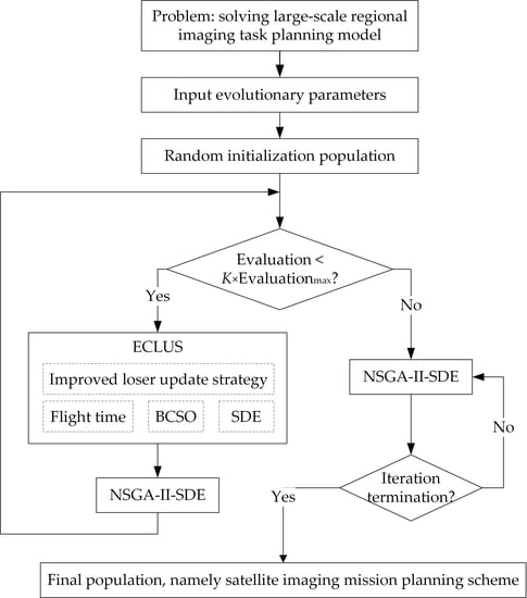
The procedure of ECL-INS-LMOA is shown in Figure 4. Firstly, some evolutionary parameters are set to prepare for the running of ECL-INS-LMOA. The evolutionary parameters of ECL-INS-LMOA include the population size , the maximum evaluations , the evolutionary strategy parameters, and the evolution process adjustment coefficient . Then, the initial population with the size of is generated through randomization. Next, the evolution process is divided into two stages through the parameter : the early and later stages. In the early stages of evolution, ECLUS is run first, followed by NSGA-II-SDE, and only NSGA-II-SDE is performed in the later stage of evolution. Finally, the final population is returned, that is, the satellite imaging mission planning scheme is returned.
The proposed ECL-INS-LMOA has the following characteristics: Firstly, an individual update strategy ECLUS with mixed decision variables and flight times is proposed to improve the convergence speed. Secondly, ECLUS and NSGA-II-SDE are run alternately to achieve complementary advantages. That is, ECLUS is used to overcome the slow convergence speed of NSGA-II-SDE in large-scale multi-objective optimization problems, and NSGA-II-SDE is used to avoid the problem of ECLUS easily falling into local optima. Thirdly, to further improve the convergence efficiency of the algorithm, SDE is used for the selection of dominant individuals in both ECLUS and NSGA-II simultaneously. Fourthly, to cater to the different evolutionary needs of the different stages of progress, ECL-INS-LMOA adopts the idea of running in two stages. ECL-INS-LMOA focuses on fast convergence while also considering global optimization in the early stage, but focuses on global optimization while also considering algorithm convergence in the later stage. ECL-INS-LMOA continuously searches for optimal solutions by combining alternating optimization with only single optimization and balancing fast convergence with global optimization in different stages until a reliable solution that meets the conditions is obtained.
4. Experiment and Analysis
4.1. Experimental Settings
4.1.1. Imaging Satellite
This paper selects the fine strip II mode of the GF3 satellite for regional imaging task planning. The satellite and sensor parameters are shown in Table 1.
4.1.2. Imaging Regions
This paper uses 100 imaging strips as the minimum limit and selects five different large regions from around the world as the regions to be imaged, namely the Congo (K), India, Australia, the United States, and Antarctica. The boundaries of each region are appropriately simplified, and the distribution of each region is shown in Figure 5. The parameters of each region are shown in Table 2.
4.1.3. Candidate Strips for Each Region
The maximum power-up time of GF3 within one cycle is about two minutes. Therefore, the maximum flight distance of GF3 during one imaging does not exceed 912 km. For the five areas to be imaged in our experiment, the north–south distance is much greater than 912 km, so the satellite cannot continuously image when passing through each region. To reasonably obtain candidate imaging strips for each region, each region is decomposed based on the maximum flight distance of the GF3, as shown in Figure 6. Only one sub-region can be imaged each time the satellite passes, and the imaging time should not exceed the maximum. Due to its special geographical location, a circular decomposition was conducted in our experiment for Antarctica. Table 3 lists the number and acquisition time of candidate strips for each region.
After the screening, the imaging time window of each candidate strip and satellite position and the velocity coordinates within it are output. This paper does not list them one by one because of the large amount of data. According to the multi-objective imaging satellite task planning model, the number of candidate strips is the number of real or binary decision variables in ECL-INS-MOEA.
4.1.4. Parameter Settings for MOEAs
In our experiments, NSGA-II, LMOCSO, and LMEA are comparative algorithms. Among them, NSGA-II is widely recognized as an MOEA with good performance for two-dimensional objective space when the decision variables of the problem are not particularly large. LMOCSO and LMEA are large-scale MOEAs based on new search strategy and decision variable grouping, respectively. The proposed ECL-INS-MOEA is a large-scale MOEA based on the new search strategy.
For the parameter settings, the population size is always set to 100 for different regions and algorithms. The number of objective function evaluations is used as a termination condition of evolution, which is different for different regions. For each region, the maximum number of evaluations for NSGA-II, LMOCSO, and ECL-INS-LMOA is the same, while the maximum number of evaluations for LMEA is more than them because LMEA requires a large amount of decision variable correlation analysis. The evaluation numbers for different regions and algorithms are shown in Table 4. The other parameter settings of comparison algorithms are consistent with their paper. In ECL-INS-LMOA, the evolution process adjustment coefficient is 0.6, the maximum flight time is 2, and the time adjustment coefficient is 0.7.
4.2. Results and Analysis
4.2.1. Verification of Particle Update Strategies in ECLUS
To demonstrate the effectiveness of ECL-INS-LMOA, we verify the effectiveness of the proposed particle update strategies through ablation experiments. The improved loser update strategy, flight time, and binary decision variable update strategy BCSO were compared with existing particle update strategies. The winner selection strategy based on SDE has not been validated because its effectiveness was studied in the literature [45]. Figure 7, Figure 8 and Figure 9 show the Congo (K) planning results of the proposed ECL-INS-LMOA with different strategies under 40,000 evaluations. Figure 7 shows the impacts of the improved loser update strategy in ECLUS and the loser update strategy in LMOCSO on the performance of ECL-INS-LMOA. Figure 8 shows the flight time strategy in ECLUS and the fixed flight time strategy on the performance of ECL-INS-LMOA. Figure 9 shows the BCSO strategy in ECLUS and the BPSO strategy on the performance of ECL-INS-LMOA. In Figure 7, Figure 8 and Figure 9, the red lines represent the results of the strategies in ECLUS, and the dotted lines of blue, green, and magenta represent the results of the comparison strategies.
In Figure 7a, the hypervolume (HV) is used to evaluate the performance of the improved loser update strategy in ECLUS and the loser update strategy in LMOCSO. The larger the HV, the better the convergence and distribution of the planning results. Therefore, from Figure 7a, it can be seen that the improved loser update strategy in ECLUS has a better impact on ECL-INS-LMOA than the loser update strategy in LMOCSO. Figure 7b shows that the improved loser update strategy in ECLUS has a better maximum coverage than the loser update strategy in LMOCSO. However, even if the number of imaging strips of the improved loser update strategy in ECLUS has a downward trend, Figure 7c shows that it is still inferior to the loser update strategy in LMOCSO. This is probably because the maximum coverage obtained by the loser update strategy in LMOCSO is small, resulting in a small number of corresponding imaging strips. In general, the improved loser update strategy in ECLUS is better than the loser update strategy in LMOCSO because the improved loser update strategy in ECLUS has advantages in HV and maximum coverage.
Figure 8 compares the flight time strategy and fixed flight time strategy from the HV, maximum coverage, and the number of imaging strips corresponding to the maximum coverage. Figure 8 shows that the strategy with flight time always achieves better results than the strategy with fixed flight time. It demonstrates the effectiveness of adopting a flight time strategy in ECLUS.
From Figure 9, it can be seen that the binary decision variable update strategy BCSO exhibits a better performance than BPSO in ECL-INS-LMOA. Although the maximum coverage advantage of BCSO in Figure 9b is small, the HV advantage in Figure 9a is marked. This is mainly because BCSO obtains better convergence and distribution binary solutions than BPSO. Figure 9c also demonstrates the effectiveness of BCSO in the number of imaging strips corresponding to the maximum coverage.
Therefore, the improved loser update strategy, the flight time strategy, and the BCSO strategy can effectively enhance the optimization ability of ECL-INS-LMOA. These three proposed strategies, together with the winner selection strategy based on SDE, ensure the excellent optimization performance of ECL-INS-LMOA in solving large-scale multi-objective optimization problems.
4.2.2. Comparison between ECL-INS-LMOA and Comparative Algorithms
In this section, Congo (K) is the region to be imaged, and the imaging task planning results obtained by ECL-INS-LMOA are compared with NSGA-II, LMOCSO, and LMEA.
- The distribution of solutions in the objective space
Figure 10 shows the distribution of non-dominated solutions obtained by four algorithms for Congo (K). According to the imaging satellite task planning model in Section 2.1, in Figure 10, the vertical axis is the objective function 1, representing the difference between 1 and the regional coverage rate. The smaller the value, the greater the regional imaging coverage rate. And the horizontal axis is the objective function 2, representing the ratio of the participating imaging strips to the total candidate strips. The smaller the value, the more efficient the utilization of the satellite. In Figure 10, the red, blue, pink, and green curves represent the distribution of non-dominated solutions obtained by ECL-INS-LMOA, LMEA, LMOCSO, and NSGA-II, respectively. Table 5 shows the values of the optimal coverage solution for each algorithm in Congo (K), as well as the corresponding coverage rate and the number of strips participating in the imaging. The gray shadow marks the maximum imaging coverage rate and the minimum number of strips participating in imaging.
From this experiment, three conclusions can be drawn: Firstly, although NSGA-II is not an algorithm designed for large-scale optimization problems, it still achieves good results in planning for Congo (K), with 135 decision variables. The regional coverage rate of NSGA-II reaches 98.88%, surpassing LMEA. But NSGA-II requires more imaging strips than other algorithms, which means that satellite resources have not been effectively saved in NSGA-II. Secondly, each algorithm can achieve good results in terms of coverage with little performance difference, not exceeding 3%. However, there is a significant difference in the required imaging strips. ECL-INS-LMOA has 29 fewer imaging strips than NSGA-II, accounting for approximately 21.5% of the candidate strips. Thirdly, ECL-INS-LMOA is significantly superior to comparison algorithms, always utilizing fewer imaging strips to achieve a higher regional coverage. ECL-INS-LMOA only uses 64 imaging strips to achieve almost full coverage of the imaging region, achieving the goal of a high regional coverage while saving satellite resources. The satellite resources are saved by 52.6%.
- 2.
- Regional coverage results
Figure 11 shows the coverage display results in Congo (K) using four different algorithms. In Figure 11, the red lines represent the simplified regional boundary of Congo (K), and the lotus root pink strips are the imaging strips obtained using various algorithms. Figure 11a shows the coverage display result of all candidate strips without any algorithm optimization, and Figure 11b–e shows the coverage display result of imaging strips optimized by NSGA-II, LMOCSO, LMEA, and ECL-INS-MOEA, respectively.
From Figure 11, the following conclusions can be drawn: Firstly, although Congo (K) can be fully covered without any algorithm optimization, the imaging strips are very dense, indicating a severe waste of satellite resources. Secondly, although each algorithm can achieve good coverage for Congo (K) and save satellite resources to varying degrees, the coverage effect varies greatly. On the one hand, there are invalid observations of imaging strips outside the region for three comparative algorithms, because the more decision variables, the more iterations the algorithm requires, and the algorithm has not yet reached the optimal within the maximum evaluation. On the other hand, due to differences in the coverage rate, there are varying degrees of gaps in the imaging schemes of the different algorithms. The imaging schemes of ECL-INS-LMOA and LMOCSO have no apparent gaps, while the imaging schemes of NSGA-II have several small gaps, and the gaps of LMEA are the most obvious. Thirdly, compared to the three comparison algorithms, ECL-INS-LMOA has fewer redundant imaging strips and no obvious gaps in the imaging region, and the distribution of imaging strips is uniform. Therefore, ECL-INS-LMOA outperforms the three comparison algorithms in terms of coverage display. In addition, it should be noted that the comparison algorithms did not obtain a better imaging scheme because the solution obtained within the maximum number of evaluations is still locally optimal. As the number of evaluations increases, all algorithms, including ECL-INS-LMOA, can obtain a better imaging scheme. However, increasing the number of evaluations means increasing the computational consumption. Moreover, the closer it is to the optimal solution, the more disproportionate the ‘cost’ and ‘benefit’ of the search solution.
- 3.
- Runtime
Table 6 shows the time consumption of ECL-INS-LMOA and the comparative algorithms for imaging planning in Congo (K). From Table 6, it can be seen that ECL-INS-LMOA has a significantly better runtime than the comparison algorithms. In addition, LMOCSO and LMEA require a longer runtime than NSGA-II. Particularly, the runtime is 10,512 s for LMEA because LMEA requires much time to analyze the decision variables. In summary, compared to the comparison algorithms, ECL-INS-LMOA not only has the best performance, but also the shortest runtime for the imaging task planning problem in Congo (K).
4.2.3. Results of ECL-INS-LMOA for Larger Regions
To verify the effectiveness of ECL-INS-LMOA in large-scale multi-objective optimization problems, four regions larger than Congo (K), including India, Australia, the United States, and Antarctica, are used as imaging regions. Figure 12 shows the distribution of non-dominated solutions obtained by each algorithm in different regions. Table 7 lists the optimal coverage solutions of ECL-INS-LMOA and the comparison algorithms in each region, as well as the corresponding regional coverage rate and the number of participating imaging strips. Figure 13 shows the coverage display of ECL-INS-LMOA in different regions. The meanings of each element in Figure 12 and Figure 13 and in Table 7 are the same as in Section 4.2.2.
From this experiment, the following conclusions can be drawn: Firstly, ECL-INS-LMOA can obtain reliable results in task planning for regions with different decision variable scales. The coverage rate always remains above 98.5%, and the percentage of participating imaging strips remains within 0.5. There is no significant decrease in performance as the number of decision variables increases. Although the coverage rate of LMOCSO in the United States is 0.15% higher than the ECL-INS-LMOA, the number of imaging strips required for LMOCSO is 140 more than that of ECL-INS-LMOA, which is too costly. ECL-INS-LMOA always achieves the best results except for this factor. Importantly, the coverage display of ECL-INS-LMOA in various regions shows an overall uniform arrangement of imaging strips, without obvious redundant observations, and only with small and limited gaps. Secondly, for NSGA-II in different regions, the proportions of participating imaging strips are around 0.6, but the coverage rates decrease, which is most evident in Antarctica with a coverage rate of only 92.30%. Thirdly, the performance of the comparison algorithm LMOCSO is relatively stable. For regions with different decision variable sizes, the coverage rate can always reach over 98%, but the percentage of participating imaging strips remains between 0.6 and 0.7. Satellite resources are wasted compared with ECL-INS-LMOA. Fourthly, for LMEA, although a higher number of evaluations is assigned based on its principles, its performance is not fully reflected.
In summary, the effectiveness of ECL-INS-LMOA in regional task planning problems with large-scale decision variables is further verified.
5. Discussion
This paper focuses on the research of large-scale multi-objective imaging satellite task planning in large areas, where large areas generally refer to areas with more than 100 imaging strips. On the one hand, it is easy to solve imaging satellite task planning in small areas using existing MOEAs. On the other hand, if the large area is decomposed into several small areas for optimization, only the local optimal solution can be obtained, limiting the acquisition of the optimal solution. We should strive to explore better imaging solutions to utilize precious satellite resources and complete imaging tasks more efficiently.
The proposed ECL-INS-LMOA achieved better optimization results than the existing MOEAs. This is because, firstly, ECL-INS-LMOA performs global optimization by directly designing more efficient search strategies and better environmental selection strategies. The global optimal solution of ECL-INS-LMOA is preserved. However, the MOEAs based on the decision variable grouping method and the decision space reduction lose the global optimal solution because of the methods of processing decision variables. Secondly, the proposed ECLUS has a faster convergence speed than the strategy in LMOCSO. The particles go directly from position to position with one evolution. On the other hand, ECLUS adjusts the flight distance by introducing flight time to accelerate convergence and avoid oscillation convergence. In addition, BCSO was proposed for updating the binary decision variables. Thirdly, ECL-INS-LMOA adopts the idea of two-stage optimization. In the early stages of evolution, ECLUS and NSGA-II-SDE run alternately, which focuses on fast convergence while balancing global optimization. In the later stage of evolution, only NSGA-II-SDE runs, which focuses on global optimization while balancing fast convergence.
ECL-INS-LMOA not only provides the optimal planning solution, but also has advantages in runtime. Firstly, ECL-INS-LMOA is based on a new search strategy without the need for additional analysis and the calculation of decision variables, so the time consumption is significantly less than LMEA. Secondly, the accelerated particle update strategy, flight time, and the winner selection strategy in ECLUS are all linear, and their increased computational cost is negligible and can be ignored. Compared with ECL-INS-LMOA, only non-dominated solutions in LMOCSO are used in particle updates per generation, which results in LMOCSO having many more evolutionary generations than ECL-INS-LMOA within the same number of objective function evaluations. As a result, the environment selection strategy of LMOCSO is executed more frequently, resulting in a lower running efficiency than the proposed ECL-INS-LMOA. Thirdly, all particles in ECL-INS-LMOA participate in winner and loser selection rather than just non-dominant particles. On the one hand, it can maintain the diversity of solutions. On the other hand, ECLUS can select winner individuals by simply comparing SDEs, and then obtain new populations by only updating the losers. In contrast, NSGA-II requires a series of operations such as competitive selection, crossover, and mutation on all individuals to obtain new populations. Therefore, ECL-INS-LMOA has a higher running efficiency than NSGA-II.
In our study, based on previous research, we specifically defined the scope of a large area, which is the area with more than 100 imaging strips. And a large-scale multi-objective optimization algorithm was specifically designed to solve large-scale task planning problems efficiently. We rarely see these in other related studies [46,47]. Although the imaging area is large in some studies, the scale of their problems may not be large. It is believed that this paper can provide some new references for large-scale satellite mission planning problems.
In addition, although the experimental satellite in this paper is only GF3, the proposed MOEA can also be applied to multi-satellite optimization problems, for example, constellation optimization [48], multi-satellite joint scheduling [49], etc. For different application problems, the goal of an MOEA is always to find the best solution to the problem. In addition to the imaging satellite task planning problem for large-scale mapping studied in this paper, there are many large-scale multi-objective optimization problems in the real world, for example, feature selection in machine learning [50,51], neural network training [52], drone-assisted camera network [53], routing problems [54,55], etc. The proposed method can also be explored for its value in different fields.
The proposed ECL-INS-LMOA focuses on innovating new search strategies, but the environmental selection strategy adopts the methods in existing papers. In the future, the environment selection strategy will be designed to enhance the performance of MOEAs. In addition, the regional mapping we are currently researching only focuses on obtaining orthophoto images of one region. In the future, we will focus on obtaining regional stereo imaging products and multi-satellite multi-region task planning problems. In summary, we will construct different imaging satellite task planning models and design corresponding solving algorithms based on specific imaging satellite task planning problems in practical applications.
6. Conclusions
To solve the imaging satellite task planning problem in large areas, we proposed ECL-INS-LMOA. ECL-INS-LMOA adopts the idea of two-stage evolution. In the early stage of evolution, the proposed ECLUS and NSGA-II-SDE are alternately run to ensure fast convergence while balancing global optimization. In the later stage of evolution, only NSGA-II-SDE is run to ensure global optimization while balancing fast convergence. To enable ECL-INS-LMOA to quickly converge to the approximate optimal solution in the early stage of evolution, we proposed ECLUS based on accelerating the particle update, introducing flight time, and proposing BCSO. This paper conducts imaging task planning experiments on five large imaging regions with a global number of imaging bands greater than 100 and compares ECL-INS-MOEA with three comparative algorithms. The experimental results show that the proposed ECL-INS-MOEA can always achieve efficient and fast convergence in different regions and obtain reliable imaging schemes. For different regions, the regional coverage rate exceeds 98.8%, the satellite resource savings exceed 50%, and the coverage is uniform, with fewer redundant observations and gaps.
With the increase in the number of satellites and the complexity and diversification of user needs, imaging satellite task planning will play an increasingly important role in both theoretical research and practical applications. We sincerely hope this paper can provide a reference for relevant research and stimulate more research interest.
Author Contributions
Conceptualization, Y.C., X.S. and G.Z.; methodology, Y.C. and X.S.; validation, Y.C., X.S. and Z.L.; formal analysis, X.S.; investigation, Y.C.; resources, Y.C.; data curation, X.S.; writing—original draft preparation, Y.C.; writing—review and editing, Y.C.; visualization, Z.L.; supervision, X.S.; project administration, G.Z.; funding acquisition, X.S. All authors have read and agreed to the published version of the manuscript.
Funding
This work was supported by the National Key R & D Program of China (2022YFB3902803) and the National Natural Science Foundation of China under grant 42171341.
Data Availability Statement
All data that support the findings of this study are available from the corresponding authors upon reasonable request.
Conflicts of Interest
The authors declare no conflict of interest.
References
- Tan, X.; Jiao, J.; Zhong, Y.; Ma, A.; Xu, Y.; Sha, Z.; Huang, F.; Wan, Y.; Hu, W. The CNRIEEEMC: A communication-navigation-remote sensing-integrated ecological environment emergency monitoring chain for tailings areas. Int. J. Appl. Earth Obs. 2022, 108, 102710. [Google Scholar] [CrossRef]
- Zhang, G.; Cui, H.; Wang, T.; Li, Z.; Jiang, B.; Li, X.; Wang, H.; Zhu, Y. Random cross-observation intensity consistency method for large-scale SAR images mosaics: An example of Gaofen-3 SAR images covering China. ISPRS J. Photogramm. 2019, 156, 215–234. [Google Scholar] [CrossRef]
- Mi, W.; Fang, Y. Intelligent remote sensing satellite and remote sensing image real-time service. Acta Geod. Cartogr. Sin. 2019, 48, 1586–1594. [Google Scholar]
- Xu, Y.; Du, B.; Zhang, L. Assessing the Threat of Adversarial Examples on Deep Neural Networks for Remote Sensing Scene Classification: Attacks and Defenses. IEEE Trans. Geosci. Remote Sens. 2021, 59, 1604–1617. [Google Scholar] [CrossRef]
- Richer-de-Forges, A.C.; Chen, Q.; Baghdadi, N.; Chen, S.; Gomez, C.; Jacquemoud, S.; Martelet, G.; Mulder, V.L.; Urbina-Salazar, D.; Vaudour, E.; et al. Remote Sensing Data for Digital Soil Mapping in French Research—A Review. Remote Sens. 2023, 15, 3070. [Google Scholar] [CrossRef]
- Zhu, B.; Bai, Y.; Zhang, Z.; He, X.; Wang, Z.; Zhang, S.; Dai, Q. Satellite Remote Sensing of Water Quality Variation in a Semi-Enclosed Bay (Yueqing Bay) under Strong Anthropogenic Impact. Remote Sens. 2022, 14, 550. [Google Scholar] [CrossRef]
- McCarthy, M.J.; Jessen, B.; Barry, M.J.; Figueroa, M.; McIntosh, J.; Murray, T.; Schmid, J.; Muller-Karger, F.E. Mapping hurricane damage: A comparative analysis of satellite monitoring methods. Int. J. Appl. Earth Obs. 2020, 91, 102134. [Google Scholar] [CrossRef]
- Xia, Z.; Li, Y.; Guo, X.; Chen, R. High-resolution mapping of water photovoltaic development in China through satellite imagery. Int. J. Appl. Earth Obs. 2022, 107, 102707. [Google Scholar] [CrossRef]
- Wang, Y.; Su, J.; Zhai, X.; Meng, F.; Liu, C. Snow Coverage Mapping by Learning from Sentinel-2 Satellite Multispectral Images via Machine Learning Algorithms. Remote Sens. 2022, 14, 782. [Google Scholar] [CrossRef]
- Chen, H.; Wang, T.; Chen, T.; Deng, W. Hyperspectral Image Classification Based on Fusing S3-PCA, 2D-SSA and Random Patch Network. Remote Sens. 2023, 15, 3402. [Google Scholar] [CrossRef]
- Lu, Z.; Shen, X.; Li, D.; Chen, Y.; Li, D. A Mission Planning Modeling Method of Multipoint Target Imaging within a Single Pass for Super-Agile Earth Observation Satellite. IEEE Syst. J. 2022, 16, 1921–1932. [Google Scholar] [CrossRef]
- Rainjonneau, S.; Tokarev, I.; Iudin, S.; Rayaprolu, S.; Pinto, K.; Lemtiuzhnikova, D.; Koblan, M.; Barashov, E.; Kordzanganeh, M.; Pflitsch, M. Quantum algorithms applied to satellite mission planning for Earth observation. arXiv 2023, arXiv:2302.07181. [Google Scholar] [CrossRef]
- Eddy, D.; Kochenderfer, M. Markov Decision Processes For Multi-Objective Satellite Task Planning. In Proceedings of the 2020 IEEE Aerospace Conference, Big Sky, MT, USA, 7–14 March 2020; pp. 1–12. [Google Scholar]
- Tian, Y.; Si, L.; Zhang, X.; Cheng, R.; He, C.; Tan, K.C.; Jin, Y. Evolutionary Large-Scale Multi-Objective Optimization: A Survey. ACM Comput. Surv. 2021, 54, 1–34. [Google Scholar] [CrossRef]
- Zhou, X.; Cai, X.; Zhang, H.; Zhang, Z.; Jin, T.; Chen, H.; Deng, W. Multi-strategy competitive-cooperative co-evolutionary algorithm and its application. Inf. Sci. 2023, 635, 328–344. [Google Scholar] [CrossRef]
- Deb, K.; Pratap, A.; Agarwal, S.; Meyarivan, T.A.M.T. A fast and elitist multi-objective genetic algorithm: NSGA-II. IEEE Trans. Evolut. Comput. 2002, 6, 182–197. [Google Scholar] [CrossRef]
- Rajani; Kumar, D.; Kumar, V. Impact of Controlling Parameters on the Performance of MOPSO Algorithm. Procedia Comput. Sci. 2020, 167, 2132–2139. [Google Scholar] [CrossRef]
- Antonio, L.M.; Coello CA, C.; Morales MA, R.; Brambila, S.G.; González, J.F.; Tapia, G.C. Co-evolutionary Operations for Large Scale Multi-objective Optimization. In Proceedings of the 2020 IEEE Congress on Evolutionary Computation (CEC), Glasgow, UK, 19–24 July 2020; pp. 1–8. [Google Scholar]
- Li, M.; Wei, J. A cooperative co-evolutionary algorithm for large-scale multi-objective optimization problems: ACM. In Proceedings of the Genetic and Evolutionary Computation Conference Companion, Kyoto, Japan, 15–19 July 2018; pp. 1716–1721. [Google Scholar]
- Cao, B.; Zhao, J.; Gu, Y.; Ling, Y.; Ma, X. Applying graph-based differential grouping for multi-objective large-scale optimization. Swarm Evol. Comput. 2020, 53, 100626. [Google Scholar] [CrossRef]
- Basu, S.; Mondal, A.; Basu, A. A Cooperative Co-evolutionary Approach for Multi-objective Optimization. In Recent Trends in Signal and Image Processing: ISSIP; Bhattacharyya, S., Mukherjee, A., Bhaumik, H., Das, S., Yoshida, K., Eds.; Springer: Singapore, 2019; pp. 57–65. [Google Scholar]
- Zhang, X.; Tian, Y.; Cheng, R.; Jin, Y. A Decision Variable Clustering-Based Evolutionary Algorithm for Large-Scale Many-Objective Optimization. IEEE Trans. Evolut. Comput. 2018, 22, 97–112. [Google Scholar] [CrossRef]
- Liu, S.; Lin, Q.; Tian, Y.; Tan, K.C. A Variable Importance-Based Differential Evolution for Large-Scale Multi-objective Optimization. IEEE Trans. Cybern. 2022, 52, 13048–13062. [Google Scholar] [CrossRef]
- Zhang, Y.; Tian, Y.; Zhang, X. Improved SparseEA for sparse large-scale multi-objective optimization problems. Complex Intell. Syst. 2023, 9, 1127–1142. [Google Scholar] [CrossRef]
- Tian, Y.; Zhang, X.; Wang, C.; Jin, Y. An Evolutionary Algorithm for Large-Scale Sparse Multi-objective Optimization Problems. IEEE Trans. Evolut. Comput. 2020, 24, 380–393. [Google Scholar] [CrossRef]
- Zille, H.; Ishibuchi, H.; Mostaghim, S.; Nojima, Y. A Framework for Large-Scale Multi-objective Optimization Based on Problem Transformation. IEEE Trans. Evolut. Comput. 2018, 22, 260–275. [Google Scholar] [CrossRef]
- He, C.; Li, L.; Tian, Y.; Zhang, X.; Cheng, R.; Jin, Y.; Yao, X. Accelerating Large-Scale Multi-objective Optimization via Problem Reformulation. IEEE Trans. Evolut. Comput. 2019, 23, 949–961. [Google Scholar] [CrossRef]
- Liu, R.; Liu, J.; Li, Y.; Liu, J. A random dynamic grouping based weight optimization framework for large-scale multi-objective optimization problems. Swarm Evol. Comput. 2020, 55, 100684. [Google Scholar] [CrossRef]
- Liu, S.; Jiang, M.; Lin, Q.; Tan, K.C. Evolutionary Large-Scale Multi-objective Optimization via Self-guided Problem Transformation. In Proceedings of the 2022 IEEE Congress on Evolutionary Computation (CEC), Padua, Italy, 18–23 July 2022; pp. 1–8. [Google Scholar]
- Liu, R.; Ren, R.; Liu, J.; Liu, J. A clustering and dimensionality reduction based evolutionary algorithm for large-scale multi-objective problems. Appl. Soft Comput. 2020, 89, 106120. [Google Scholar] [CrossRef]
- Ji, W.; Yue, Y.; Wang, X.; Lin, P. Large-scale Multi-objective Natural Computation Based on Dimensionality Reduction and Clustering. J. Syst. Simul. 2023, 35, 41–56. [Google Scholar]
- Tan, Z.; Wang, H.; Liu, S. Multi-stage dimension reduction for expensive sparse multi-objective optimization problems. Neurocomputing 2021, 440, 159–174. [Google Scholar] [CrossRef]
- Tian, Y.; Lu, C.; Zhang, X.; Tan, K.C.; Jin, Y. Solving large-scale multi-objective optimization problems with sparse optimal solutions via unsupervised neural networks. IEEE Trans. Cybern. 2020, 51, 3115–3128. [Google Scholar] [CrossRef]
- He, C.; Cheng, R.; Yazdani, D. Adaptive Offspring Generation for Evolutionary Large-Scale Multi-objective Optimization. IEEE Trans. Syst. Man Cybern. Syst. 2022, 52, 786–798. [Google Scholar] [CrossRef]
- Liang, Z.; Li, Y.; Wan, Z. Large-scale many-objective optimization driven by distributional adversarial networks. arXiv 2020, arXiv:2003.07013. [Google Scholar]
- He, C.; Huang, S.; Cheng, R.; Tan, K.C.; Jin, Y. Evolutionary multi-objective optimization driven by generative adversarial networks (GANs). IEEE Trans. Cybern. 2020, 51, 3129–3142. [Google Scholar] [CrossRef] [PubMed]
- Kropp, I.; Nejadhashemi, A.P.; Deb, K. Improved Evolutionary Operators for Sparse Large-Scale Multi-objective Optimization Problems. IEEE Trans. Intell. Transp. Syst. 2023, 1. [Google Scholar] [CrossRef]
- Ding, Z.; Chen, L.; Sun, D.; Zhang, X. A multi-stage knowledge-guided evolutionary algorithm for large-scale sparse multi-objective optimization problems. Swarm Evol. Comput. 2022, 73, 101119. [Google Scholar] [CrossRef]
- Zhang, Y.; Wang, G.; Li, K.; Yeh, W.; Jian, M.; Dong, J. Enhancing MOEA/D with information feedback models for large-scale many-objective optimization. Inf. Sci. 2020, 522, 1–16. [Google Scholar] [CrossRef]
- Tian, Y.; Chen, H.; Ma, H.; Zhang, X.; Tan, K.C.; Jin, Y. Integrating Conjugate Gradients Into Evolutionary Algorithms for Large-Scale Continuous Multi-Objective Optimization. IEEE/CAA J. Autom. Sin. 2022, 9, 1801–1817. [Google Scholar] [CrossRef]
- Cheng, R.; Jin, Y. A Competitive Swarm Optimizer for Large Scale Optimization. IEEE Trans. Cybern. 2015, 45, 191–204. [Google Scholar] [CrossRef] [PubMed]
- Tian, Y.; Zheng, X.; Zhang, X.; Jin, Y. Efficient Large-Scale Multi-objective Optimization Based on a Competitive Swarm Optimizer. IEEE Trans. Cybern. 2020, 50, 3696–3708. [Google Scholar] [CrossRef]
- Chen, Y.; Xu, M.; Shen, X.; Zhang, G.; Lu, Z.; Xu, J. A Multi-Objective Modeling Method of Multi-Satellite Imaging Task Planning for Large Regional Mapping. Remote Sens. 2020, 12, 344. [Google Scholar] [CrossRef]
- Cheng, R.; Jin, Y.; Olhofer, M. Test Problems for Large-Scale Multi-objective and Many-Objective Optimization. IEEE Trans. Cybern. 2017, 47, 4108–4121. [Google Scholar] [CrossRef]
- Li, M.; Yang, S.; Liu, X. Shift-Based Density Estimation for Pareto-Based Algorithms in Many-Objective Optimization. IEEE Trans. Evolut. Comput. 2014, 18, 348–365. [Google Scholar] [CrossRef]
- Xu, Y.; Liu, X.; He, R.; Chen, Y. Multi-satellite scheduling framework and algorithm for very large area observation. Acta Astronaut. 2020, 167, 93–107. [Google Scholar] [CrossRef]
- Gu, Y.; Han, C.; Chen, Y.; Liu, S.; Wang, X. Large Region Targets Observation Scheduling by Multiple Satellites Using Resampling Particle Swarm Optimization. IEEE Trans. Aerosp. Electron. Syst. 2023, 59, 1800–1815. [Google Scholar] [CrossRef]
- Zhao, S.; Wang, Y.; Zhang, Y.; Zheng, K. Research Progress and Prospect of Satellite Constellation Optimization Design. J. Phys. Conf. Ser. 2023, 2457, 12045. [Google Scholar] [CrossRef]
- Long, J.; Wu, S.; Han, X.; Wang, Y.; Liu, L. Autonomous Task Planning Method for Multi-Satellite System Based on a Hybrid Genetic Algorithm. Aerospace 2023, 10, 70. [Google Scholar] [CrossRef]
- Li, H.; He, F.; Chen, Y.; Pan, Y. MLFS-CCDE: Multi-objective large-scale feature selection by cooperative co-evolutionary differential evolution. Memetic Comput. 2021, 13, 1–18. [Google Scholar] [CrossRef]
- Abdollahzadeh, B.; Gharehchopogh, F.S. A multi-objective optimization algorithm for feature selection problems. Eng. Comput. 2022, 38, 1845–1863. [Google Scholar] [CrossRef]
- Mishra, V.; Kane, L. A survey of designing convolutional neural network using evolutionary algorithms. Artif. Intell. Rev. 2023, 56, 5095–5132. [Google Scholar] [CrossRef]
- Cao, B.; Li, M.; Liu, X.; Zhao, J.; Cao, W.; Lv, Z. Many-Objective Deployment Optimization for a Drone-Assisted Camera Network. IEEE Trans. Netw. Sci. Eng. 2021, 8, 2756–2764. [Google Scholar] [CrossRef]
- Yang, X.; Yang, Y.; Qu, D.; Chen, X.; Li, Y. Multi-Objective Optimization of Evacuation Route for Heterogeneous Passengers in the Metro Station Considering Node Efficiency. IEEE Trans. Intell. Transp. Syst. 2023, 1–14. [Google Scholar] [CrossRef]
- Zhang, L.; Liu, T.; Ding, X. Large-Scale WSNs Resource Scheduling Algorithm in Smart Transportation Monitoring Based on Differential Ion Coevolution and Multi-Objective Decomposition. IEEE Trans. Intell. Transp. Syst. 2022, 1–10. [Google Scholar] [CrossRef]
Figure 1.
Updating trajectories of the loser with two-dimensional decision variables. (a) Updating trajectories of CSO. (b) Updating trajectories of LOMCSO.
Figure 1.
Updating trajectories of the loser with two-dimensional decision variables. (a) Updating trajectories of CSO. (b) Updating trajectories of LOMCSO.

Figure 2.
Improved particle update strategy.

Figure 3.
The selection of the winner, (a) Shift-based density estimation, (b) Crowding distance.

Figure 4.
The procedure of ECL-INS-LMOA.

Figure 5.
Distribution of imaging regions.

Figure 6.
Region decomposition for obtaining candidate imaging strips. (a) Congo (K); (b) India; (c) Australia; (d) the United States; (e) Antarctica.
Figure 6.
Region decomposition for obtaining candidate imaging strips. (a) Congo (K); (b) India; (c) Australia; (d) the United States; (e) Antarctica.

Figure 7.
Strategy comparison between improved loser update strategy and loser update strategy in LMOCSO. (a) The changing HV with evolution; (b) the changing maximum coverage with evolution; and (c) the number of imaging strips corresponding to the maximum coverage per generation evolution.
Figure 7.
Strategy comparison between improved loser update strategy and loser update strategy in LMOCSO. (a) The changing HV with evolution; (b) the changing maximum coverage with evolution; and (c) the number of imaging strips corresponding to the maximum coverage per generation evolution.

Figure 8.
Strategy comparison between flight time and fixed flight time. (a) The changing HV with evolution; (b) the changing maximum coverage with evolution; and (c) the number of imaging strips corresponding to the maximum coverage per generation evolution.
Figure 8.
Strategy comparison between flight time and fixed flight time. (a) The changing HV with evolution; (b) the changing maximum coverage with evolution; and (c) the number of imaging strips corresponding to the maximum coverage per generation evolution.

Figure 9.
Strategy comparison between BCSO and BPSO. (a) The changing HV with evolution; (b) the changing maximum coverage with evolution; and (c) the number of imaging strips corresponding to the maximum coverage per generation evolution.
Figure 9.
Strategy comparison between BCSO and BPSO. (a) The changing HV with evolution; (b) the changing maximum coverage with evolution; and (c) the number of imaging strips corresponding to the maximum coverage per generation evolution.

Figure 10.
Distribution of planning solution in Congo (K) using different algorithms.

Figure 11.
Coverage displays of task planning results in Congo (K) for different algorithms. (a) No optimization; (b) NSGA-II; (c) LMOCSO; (d) LMEA; (e) ECL-INS-LMOA.
Figure 11.
Coverage displays of task planning results in Congo (K) for different algorithms. (a) No optimization; (b) NSGA-II; (c) LMOCSO; (d) LMEA; (e) ECL-INS-LMOA.


Figure 12.
The distribution of non-dominated solutions obtained by each algorithm in different regions. (a) India; (b) Australia; (c) the United States; (d) Antarctica.
Figure 12.
The distribution of non-dominated solutions obtained by each algorithm in different regions. (a) India; (b) Australia; (c) the United States; (d) Antarctica.

Figure 13.
Coverage displays of ECL-INS-LMOA in different regions. (a) India; (b) Australia; (c) the United States; (d) Antarctica.
Figure 13.
Coverage displays of ECL-INS-LMOA in different regions. (a) India; (b) Australia; (c) the United States; (d) Antarctica.


Table 1.
The parameters of Gaofen-3.
| Satellite | Gaofen-3 |
|---|---|
| Launch Time | 10 August 2016 |
| Orbit Type | Repeat sun-synchronous orbit |
| Orbital Altitude (km) | 755 |
| Imaging Mode | Fine strip II |
| Swing Ability | 19–50° |
| Spatial Resolution (m) | 10 |
| Swath Width (km) | 100 |
| Band | C |
| Polarization | Dual polarization |
Table 2.
Imaging area parameters.
| Region | Congo (K) | India | Australia | USA | Antarctica |
|---|---|---|---|---|---|
| Area (10,000 square km) | 234.5 | 298.0 | 774.1 | 936.4 | 1424.5 |
| Ranking in world | 11 | 7 | 6 | 4 | - |
Table 3.
Candidate imaging strip information for each region.
| Region | Sub-Region | Imaging Time | Number of Candidate Stripes | Number of Real/Binary Decision Variables |
|---|---|---|---|---|
| Congo (K) | 1 | 1 December 2019–31 December 2019 | 41 | 135 |
| 2 | 1 January 2020–31 January 2020 | 52 | ||
| 3 | 1 February 2020–29 February 2020 | 42 | ||
| India | 1 | 1 December 2019–31 December 2019 | 37 | 264 |
| 2 | 1 January 2020–31 January 2020 | 80 | ||
| 3 | 1 February 2020–29 February 2020 | 74 | ||
| 4 | 1 March 2020–31 March 2020 | 44 | ||
| 5 | 1 April 2020–30 April 2020 | 29 | ||
| Australia | 1 | 1 December 2019–31 December 2019 | 64 | 411 |
| 2 | 1 January 2020–31 January 2020 | 97 | ||
| 3 | 1 February 2020–29 February 2020 | 98 | ||
| 4 | 1 March 2020–31 March 2020 | 105 | ||
| 5 | 1 April 2020–30 April 2020 | 47 | ||
| The United States | 1 | 1 December 2019–31 December 2019 | 115 | 491 |
| 2 | 1 January 2020–31 January 2020 | 131 | ||
| 3 | 1 February 2020–29 February 2020 | 118 | ||
| 4 | 1 March 2020–31 March 2020 | 104 | ||
| 5 | 1 April 2020–20 April 2020 | 23 | ||
| Antarctica | 1 | 19 December 2019–20 December 2019 | 20 | 798 |
| 2 | 20 December 2019–26 December 2019 | 96 | ||
| 3 | 26 December 2019–1 January 2020 | 99 | ||
| 4 | 1 January 2020–7 January 2020 | 91 | ||
| 5 | 7 January 2020–13 January 2020 | 91 | ||
| 6 | 13 January 2020–23 January 2020 | 163 | ||
| 7 | 23 January 2020–3 February 2020 | 79 | ||
| 8 | 3 February 2020–16 February 2020 | 139 | ||
| 9 | 16 February 2020–28 February 2020 | 20 |
Table 4.
Iteration termination evaluation times of each algorithm.
| Region | Number of Decision Variables | Evaluation Times of Objective Function | |||
|---|---|---|---|---|---|
| NSGA-II | LMOCSO | LMEA | ECL-INS-LMOA | ||
| Congo (K) | 135 | 48,000 | 48,000 | 160,000 | 48,000 |
| India | 264 | 70,000 | 70,000 | 1,320,000 | 70,000 |
| Australia | 411 | 100,000 | 100,000 | 2,000,000 | 100,000 |
| The United States | 491 | 130,000 | 130,000 | 2,000,000 | 130,000 |
| Antarctica | 798 | 160,000 | 160,000 | 2,100,000 | 160,000 |
Table 5.
Optimal coverage solutions in Congo (K) for different algorithms.
| Algorithm | Objective Function 1 | Coverage Rate | Objective Function 2 | Number of Imaging Strips |
|---|---|---|---|---|
| LMEA | 0.02902 | 97.10% | 0.60000 | 81 |
| LMOCSO | 0.00067 | 99.93% | 0.62963 | 85 |
| NSGA-II | 0.01120 | 98.88% | 0.68889 | 93 |
| ECL-INS-LMOA | 0.00018 | 99.98% | 0.47407 | 64 |
Table 6.
Runtimes of different algorithms in Congo (K) (s).
| Algorithm | NSGA-II | LMOCSO | LMEA | ECL-INS-LMOA |
|---|---|---|---|---|
| Calculation time of objective functions | 1.2992 | |||
| Total optimization time | 7.7601 × 10² | 1.5365 × 10³ | 1.0512 × 10⁴ | 5.3960 × 10² |
Table 7.
Optimal coverage solutions of each algorithm in different regions.
| Region | Algorithm | Objective Function 1 | Coverage Rate | Objective Function 2 | Number of Imaging Strips |
|---|---|---|---|---|---|
| India | LMEA | 0.01037 | 98.96% | 0.38636 | 102 |
| LMOCSO | 0.00389 | 99.61% | 0.62121 | 164 | |
| NSGA-II | 0.01418 | 98.58% | 0.65530 | 173 | |
| ECSO-NSGA-II | 0.00113 | 99.89% | 0.36364 | 96 | |
| Australia | LMEA | 0.03913 | 96.09% | 0.54745 | 225 |
| LMOCSO | 0.01430 | 98.57% | 0.67153 | 276 | |
| NSGA-II | 0.03689 | 96.31% | 0.55961 | 230 | |
| ECSO-NSGA-II | 0.00736 | 99.26% | 0.43552 | 179 | |
| The United States | LMEA | 0.02598 | 97.40% | 0.42974 | 211 |
| LMOCSO | 0.00542 | 99.46% | 0.65173 | 320 | |
| NSGA-II | 0.02597 | 97.40% | 0.57434 | 282 | |
| ECSO-NSGA-II | 0.00688 | 99.31% | 0.36660 | 180 | |
| Antarctica | LMEA | 0.04870 | 95.13% | 0.51504 | 411 |
| LMOCSO | 0.01726 | 98.27% | 0.68797 | 549 | |
| NSGA-II | 0.07696 | 92.30% | 0.58647 | 468 | |
| ECSO-NSGA-II | 0.01158 | 98.84% | 0.36591 | 292 |
Disclaimer/Publisher’s Note: The statements, opinions and data contained in all publications are solely those of the individual author(s) and contributor(s) and not of MDPI and/or the editor(s). MDPI and/or the editor(s) disclaim responsibility for any injury to people or property resulting from any ideas, methods, instructions or products referred to in the content. |
© 2023 by the authors. Licensee MDPI, Basel, Switzerland. This article is an open access article distributed under the terms and conditions of the Creative Commons Attribution (CC BY) license (https://creativecommons.org/licenses/by/4.0/).
Share and Cite
MDPI and ACS Style
Chen, Y.; Shen, X.; Zhang, G.; Lu, Z. Large-Scale Multi-Objective Imaging Satellite Task Planning Algorithm for Vast Area Mapping. Remote Sens. 2023, 15, 4178. https://doi.org/10.3390/rs15174178
AMA Style
Chen Y, Shen X, Zhang G, Lu Z. Large-Scale Multi-Objective Imaging Satellite Task Planning Algorithm for Vast Area Mapping. Remote Sensing. 2023; 15(17):4178. https://doi.org/10.3390/rs15174178
Chicago/Turabian StyleChen, Yaxin, Xin Shen, Guo Zhang, and Zezhong Lu. 2023. "Large-Scale Multi-Objective Imaging Satellite Task Planning Algorithm for Vast Area Mapping" Remote Sensing 15, no. 17: 4178. https://doi.org/10.3390/rs15174178
Note that from the first issue of 2016, this journal uses article numbers instead of page numbers. See further details here.