
Improved Bootstrap Method Based on RBF Neural Network for Reliability Assessment
1
Department of Basic Courses, Naval University of the Engineering, Wuhan 430033, China
2
College of Naval Architecture and Ocean Engineering, Naval University of the Engineering, Wuhan 430033, China
*
Author to whom correspondence should be addressed.
Appl. Sci. 2024, 14(7), 2901; https://doi.org/10.3390/app14072901
Submission received: 26 February 2024
/
Revised: 19 March 2024
/
Accepted: 28 March 2024
/
Published: 29 March 2024
(This article belongs to the Special Issue Advances and Challenges in Reliability and Maintenance Engineering)
Abstract
:The investigation of the reliability of long-life equipment is typically hindered by the lack of experimental data, which makes accurate assessments challenging. To address this problem, a bootstrap method based on the improved RBF (radial basis function) neural network is proposed. This method utilizes the exponential function to modify the conventional empirical distribution function and fit right-tailed data. In addition, it employs the RBF radial basis neural network to obtain the distribution characteristics of the original samples and then constructs the neighborhood function to generate the input network. The expanded sample is used to estimate the scale and shape parameters of the Weibull distribution and obtain the estimated value of the MTBF (mean time between failures). The bias correction method is then used to obtain the interval estimate for the MTBF. Subsequently, a simulation experiment is conducted based on the failure data of a CNC (computer numerical control) machine tool to verify the effect of this method. The results show that the accuracy of the MTBF point estimation and interval estimation obtained using the proposed method is superior to those of the original and conventional bootstrap methods, which is of major significance to engineering applications.
1. Introduction
Reliability refers to the ability of a product to fulfill a particular function within a predetermined period and under specified conditions. It is an important index that is used to determine the performance of a product. With the advancements in manufacturing technology, the reliability of computer numerical control (CNC) machine tools and other equipment is continuously improving, and failure data are scarce. Therefore, conventional approaches based on large sample data have limited applicability in current reliability research. The accurate estimation of the reliability index of a product using limited sample data remains a key challenge in reliability research.
Currently, two main methods exist to address the problem of an insufficient sample size in reliability assessment. The first approach uses information fusion methods to fuse multiple sources of a priori information to increase the information available for assessment, thereby achieving a higher parameter accuracy. The Bayes method is an example and has been widely used in recent years for parameter estimation with the Weibull distribution [1,2,3]. Although it yields accurate estimation results using fewer samples, it requires a greater amount of a priori information and is affected by subjective factors. The second approach expands small data samples into large data samples. This method can also achieve accurate estimation results using fewer samples; however, the a priori information requirements are higher, and the influence of subjective factors is non-negligible. The bootstrap method is a typical example of this approach, and it is favored by scholars due to its simplicity and convenience. However, it completely relies on the original samples, and, if these samples are not sufficiently informative, the estimation results will have a large error. Therefore, several researchers have studied and improved the bootstrap method, which was originally proposed by Efron [4]. This body of work can be categorized into advancements in methodological accuracy, application to limited datasets, and refinements for enhanced sample representation.
Firstly, concerning methodological accuracy, Picheny et al. [5] leveraged the bootstrap method for reliability estimation and analyzed the relationship between estimation accuracy and confidence level. They established that the bootstrap method attains a higher accuracy at the 95% confidence level. Building on the bootstrap’s foundational use, Amalnerkar et al. [6] integrated the bootstrap information criterion with bootstrap resampling to estimate reliability from limited subsample data, demonstrating the method’s effectiveness even with small subsamples.
Secondly, addressing the challenges of using the bootstrap method with limited data, Zhang et al. [7] proposed an improved bootstrap approach that ensures that expanded samples remain within the mean error of the original samples, thereby maintaining result reliability without altering the probability distribution. Similarly, Sun et al. [8] developed an enhanced Bayes bootstrap method that applies an interpolation method to construct a neighborhood function, facilitating the expansion of the original sample size.
Lastly, on the front of sample representation refinement, Zhao et al. [9] tackled the issue of large deviations between the empirical distribution function of original samples and the actual distribution. They employed a B-spline function to derive an empirical distribution more suited for sampling, which proved to meet the accuracy requirements of engineering applications. Additionally, Tang et al. [10] introduced a bootstrap data expansion technique using the radial basis neural network for assessing small-sample reliability data, validating that the sample distribution characteristics closely mirror the actual distribution.
The Weibull distribution has been demonstrated to effectively model lifetime distributions in several practical engineering problems based on failure data for mechanical components, electronic components, and biological tissues. It can also describe different types of failure rate distributions, ranging from exponential to Rayleigh distributions. Due to the well-characterized nature of the Weibull distribution, it is widely used and among the most successful life models [11]. There is an extensive literature on the applications and analytical methods of Weibull models, such as the recent studies by Thanh Thach et al. [12], Piña Monarrez et al. [13], and Almarashi et al. [14].
This paper proposes an improved bootstrap method using the radial basis neural network based on the research by Tang et al. [10]. Particularly, the exponential function is used to modify the empirical distribution function, and a neighborhood function is introduced to widen the range of values of the expansion samples. Moreover, the confidence interval of the parameters of the Weibull life distribution is estimated using the bias correction method. Finally, the proposed method is validated using failure data obtained from CNC machine tools.
2. Weibull Distribution
The Weibull distribution is extensively used in the field of reliability engineering. It applies to several types of atypical electronic products [15] and can adequately describe the different cases of bathtub curves. Moreover, it can simplify the calculation steps using a transformed functional form.
Several studies on the Weibull distribution have shown that, if a localized failure results in the malfunctioning of the entire system, the life of such a system generally obeys the Weibull distribution.
The probability density function (PDF) of the two-parameter Weibull distribution is the following:
where is the shape parameter, is the scale parameter, and is the time.
The cumulative distribution function is as follows:
The reliability function is the following:
The lapse rate function is as follows:
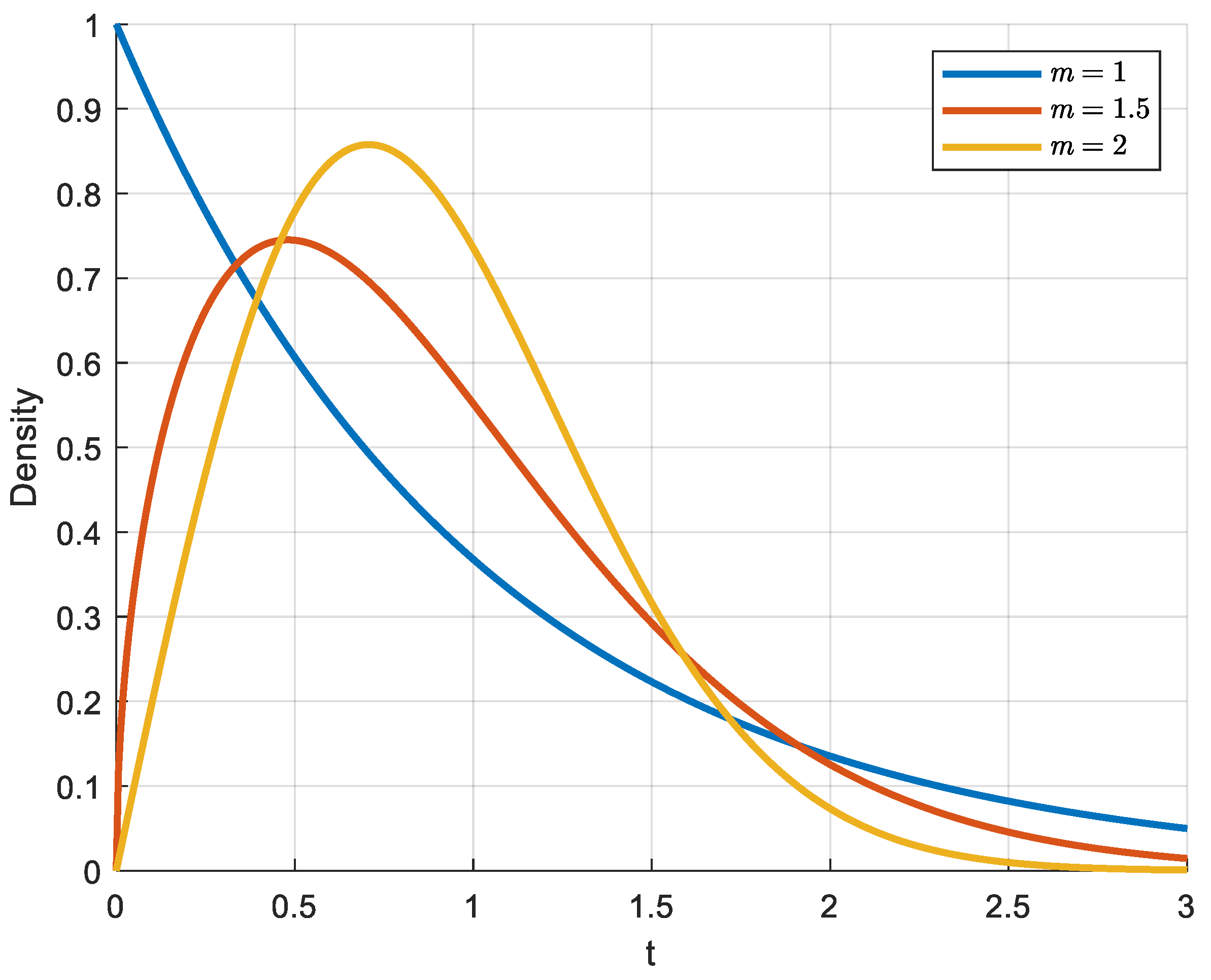
The shape parameter has a strong influence on the Weibull distribution.
Specifically, when , the density function and the failure rate function are both decreasing functions, suggesting early failure.
When , the Weibull distribution is exponential.
Finally, when , the density function curve has a single peak, and, when , the density function curve has a single symmetrical peak, resembling a normal distribution. The failure rate is an increasing function, which suggests wear failure of the product. The density functional curves for different shape parameters ( fixed) are shown in Figure 1.
3. Bootstrap Methodology and Its Improvement
3.1. Bootstrap Approach
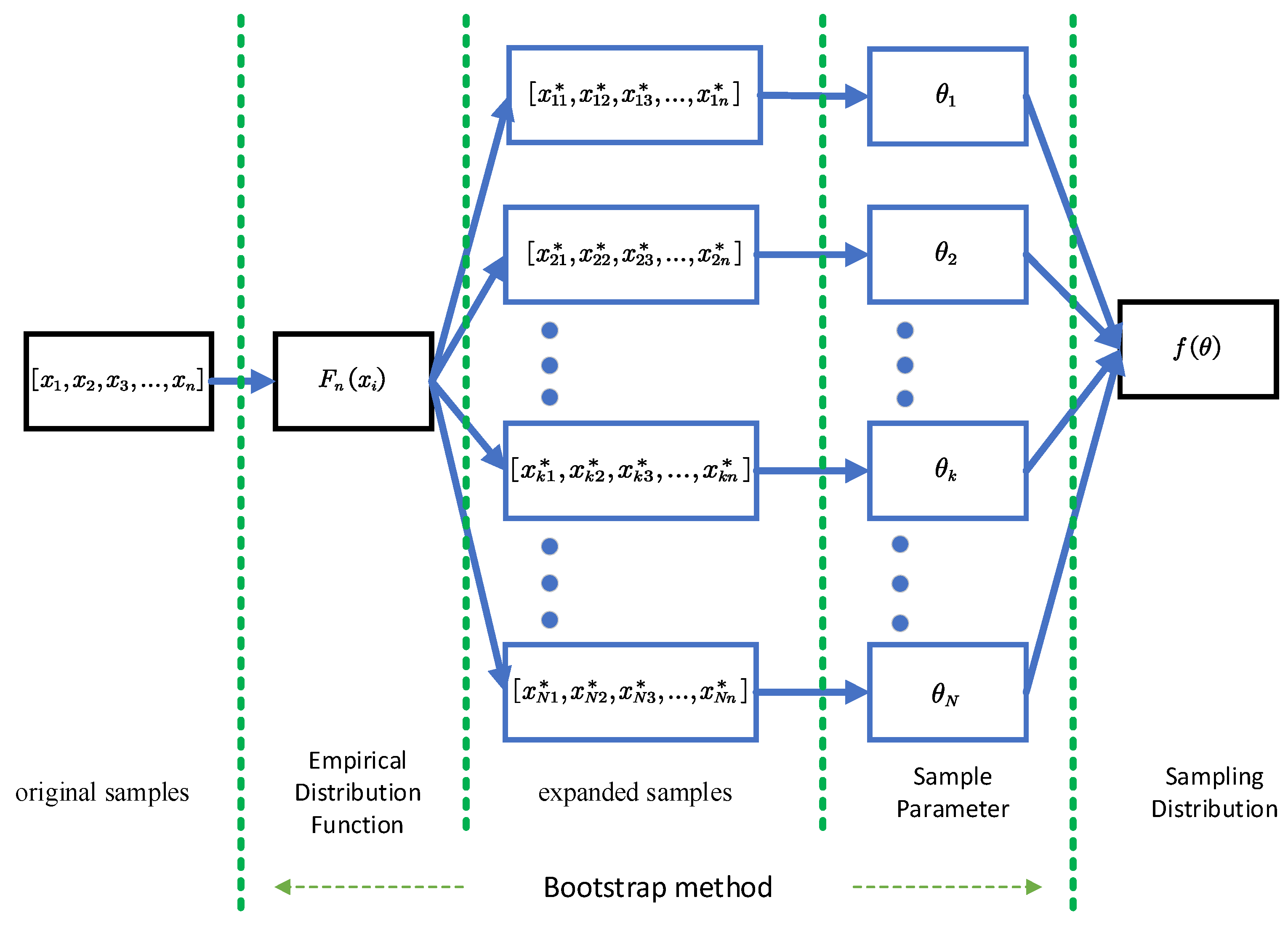
Let be a set of random variables with a joint distribution . To estimate the overall parameter , it is generally possible to obtain a sample-based estimate . The basic concept underlying the bootstrap method is that, given , one can construct an estimate of and then regenerate a set of random variables from the distribution . If is the best estimate of , then the relationship between and is adequately represented by the relationship between and , where is called the empirical distribution function of the bootstrap method. This step can be repeated several times to obtain multiple estimates from the reconstructed data according to an estimation equation, as that for . The metrics for measuring the accuracy of the estimator can then be obtained (e.g., using the Bayes method). The principle of the bootstrap method is illustrated in Figure 2. and the procedure is as follows.
The order statistics of the samples can be obtained by arranging the original samples in descending order, i.e., , where and .
When the parameters of the estimated distribution are unknown and if the value of the cumulative distribution function at is , then the empirical distribution function of the original sample assuming equal probability sampling is
The simulation-based method for generating random samples that obey the empirical distribution function is as follows:
- Uniformly distributed pseudo-random numbers in the interval [0, 1] are generated;
- Let , where is rounded down;
- Let , where is the desired random sample.
A review of existing studies and experimental simulations revealed that the resampling of the data in the bootstrap method relies on the original samples. Therefore, the random samples generated are typically not representative of the whole population, and the estimates obtained may be biased. Moreover, the bootstrap method may not be robust enough in terms of the margins (i.e., extremes) of the data distribution, because the extremes may be over-represented or under-represented in the generated random samples generated. The bootstrap method is, therefore, not reasonable when processing small subsamples of data. There are two main reasons for this. First, when is used to generate random samples, the sample values are extracted from the original sample with a medium probability to form an expanded sample. The resulting sample’s empirical function , which is used to fit the head and the tail samples, is inadequate. Consequently, the samples generated according to are not satisfactorily random. Second, because the generated random samples are limited by the minimum and maximum values [16] and the values of random samples can only be extracted from the head and tail samples using limited subsample data, the bootstrap method is ineffective.
Moreover, as the values of the random samples can only be obtained from the range of the original samples, the samples are not adequately random [17,18]. Therefore, this paper aims to address these two problems. For the first problem, the exponential distribution function is used to perform the correction of the sample’s empirical function, as the life of electronic products essentially obeys an exponential distribution [19]. For the second problem, based on the corrected empirical distribution function, the radial basis function (RBF) neural network is used to fit the original empirical distribution and obtain the continuous distribution characteristics of the original sample. The input set of the RBF neural network is then obtained using the neighborhood sampling method to ensure that the expanded sample is not limited by the original data. Thus, the expanded sample resembles the actual distribution of the original sample.
3.2. Modified Exponential Sample Empirical Function
For long-life devices such as electronic products, the failure rate rarely increases due to fatigue or wear and tear. Therefore, the tail of the cumulative distribution function of failure can be approximated by the exponential function, with a mean equal to the sample mean [19,20,21]. In this study, the exponential distribution function is utilized to fit the samples and correct the empirical distribution function . The exponential distribution function generally has a good fitting property, which can better estimate the unobserved data points and reduce the influence of random errors on the results. The steps involved are as follows.
- A linear empirical distribution function is introduced for each segment before samples, where is the total number of samples, and is the number of tail samples.
- The samples after are fitted using an exponential distribution with the same mean as the original sample. Considering integer values below five for results in a smaller variance in the right tail fit [22]. The modified empirical distribution function for the samples iswhere . The simulation-based method for generating random samples that obey the modified empirical distribution function involves the following steps:
- Uniformly distributed pseudo-random numbers in the interval [0, 1] are generated;
- If , then is the desired random number; otherwise, go to step (3);
- Let , and ; then,is the desired random number.
3.3. Simulation Verification
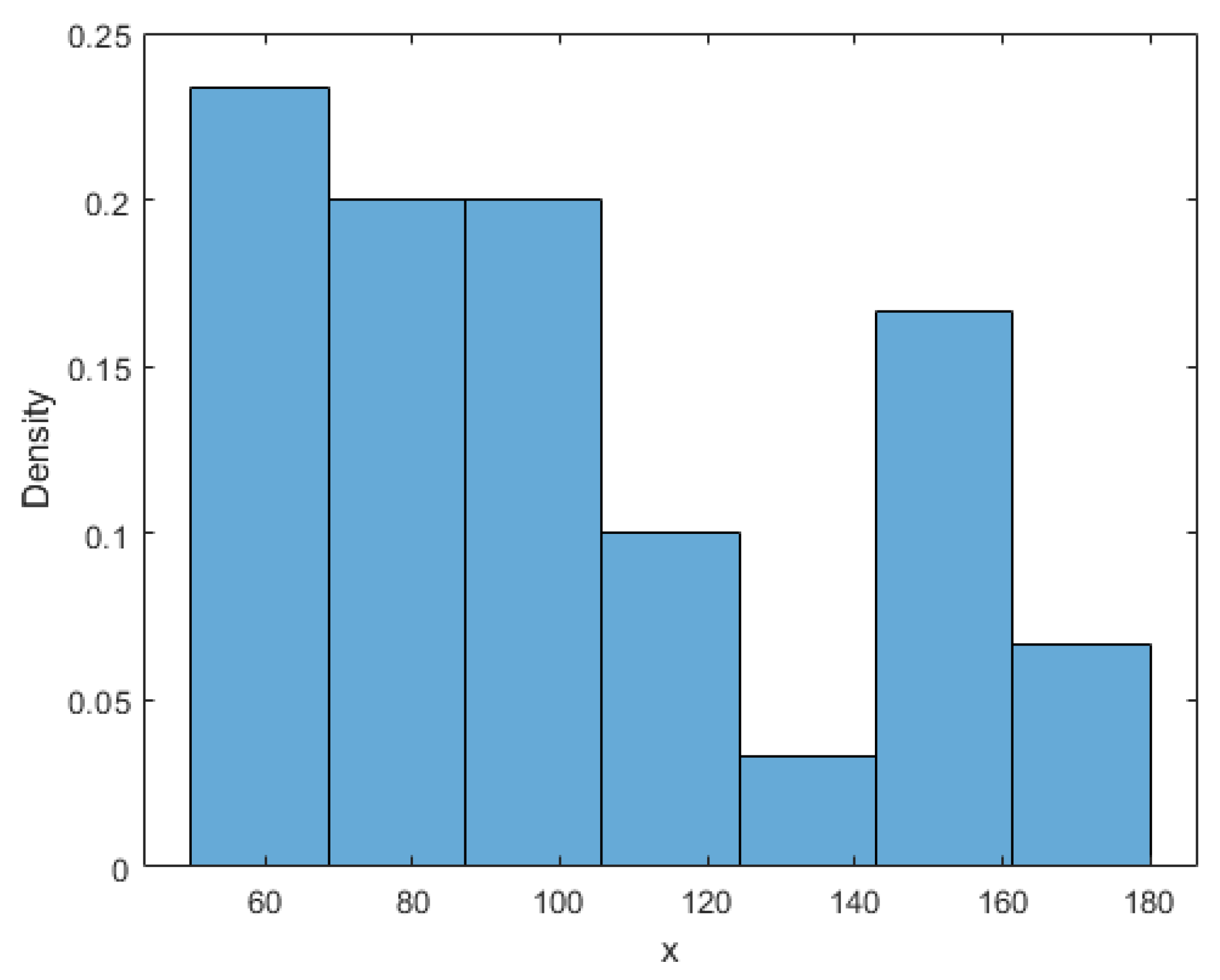
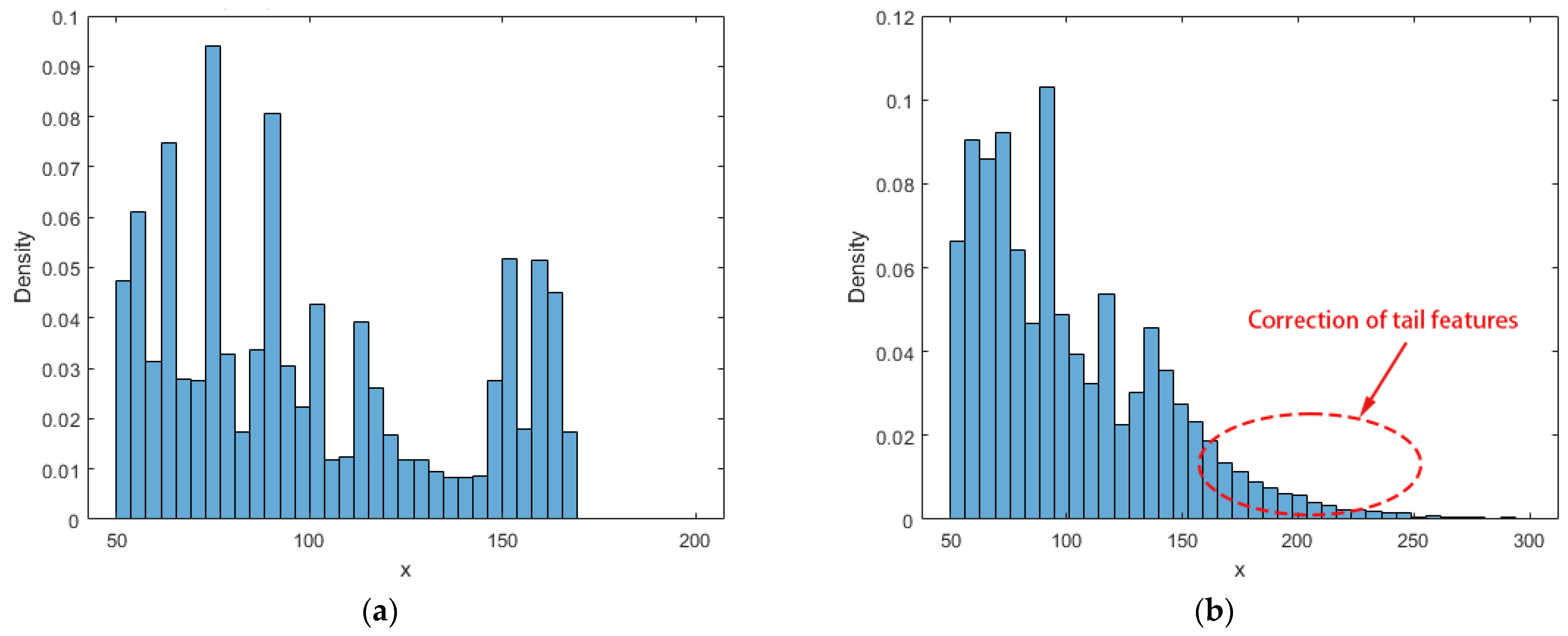
Let the original sample dataset be generated using the exponential distribution with a mean of 100, with a sample capacity of . The sample dataset is summarized in Table 1, and its distribution is shown in Figure 3. Sampling is performed times, and is expanded into , with a sample capacity of 1000 × 30. The classical bootstrap method is used to obtain the expanded sample , and the improved bootstrap method is used to obtain the expanded sample . Their distributions are shown in Figure 4. The distribution characteristics of are analyzed, and the results are as follows.
The original samples obey the exponential distribution, and expanded samples are obtained using the bootstrap method by correcting the empirical distribution function . Evidently, compared to the conventional bootstrap method, the tails resulting from the correction of the exponential function have an overall distribution that is more in line with the characteristics of the original distribution. The range of the augmented samples generated using the modified bootstrap method increases, which improves the randomness of the augmented samples (Figure 4).
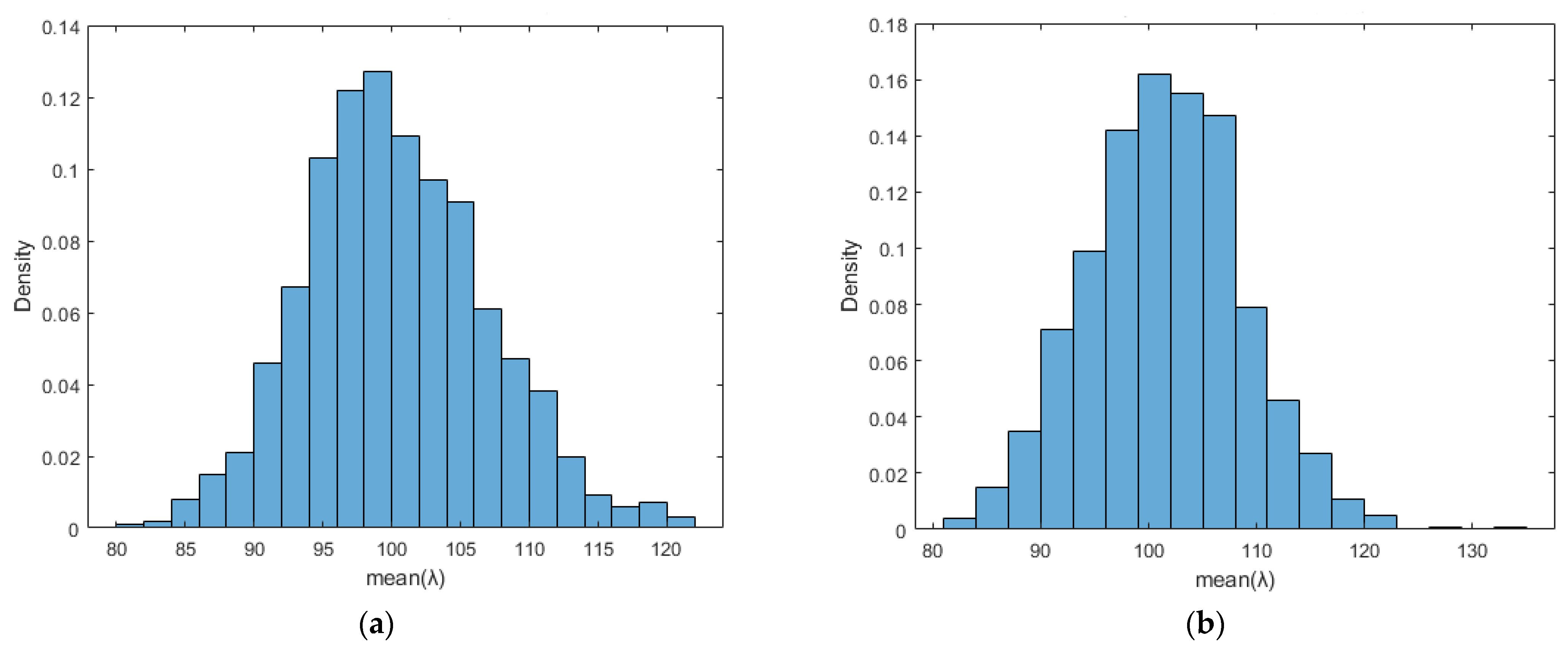
The distribution of the expanded samples in Figure 4, the parameter distribution of the expanded samples in Figure 5, and the estimation of the parameter in Table 2 show that the improved bootstrap method overestimates the sample parameter . There is an insignificant difference in terms of the accuracy when compared with the conventional method. However, the confidence interval generated by the improved method is markedly narrower compared to that produced by the conventional method, thereby demonstrating a significant superiority in the estimation of confidence intervals. Therefore, this study uses the improved bootstrap method in conjunction with the RBF neural network for sample expansion.
4. Improved Bootstrap Data Expansion Methodology Based on RBF Neural Network and Reliability Assessment
4.1. RBF Neural Network
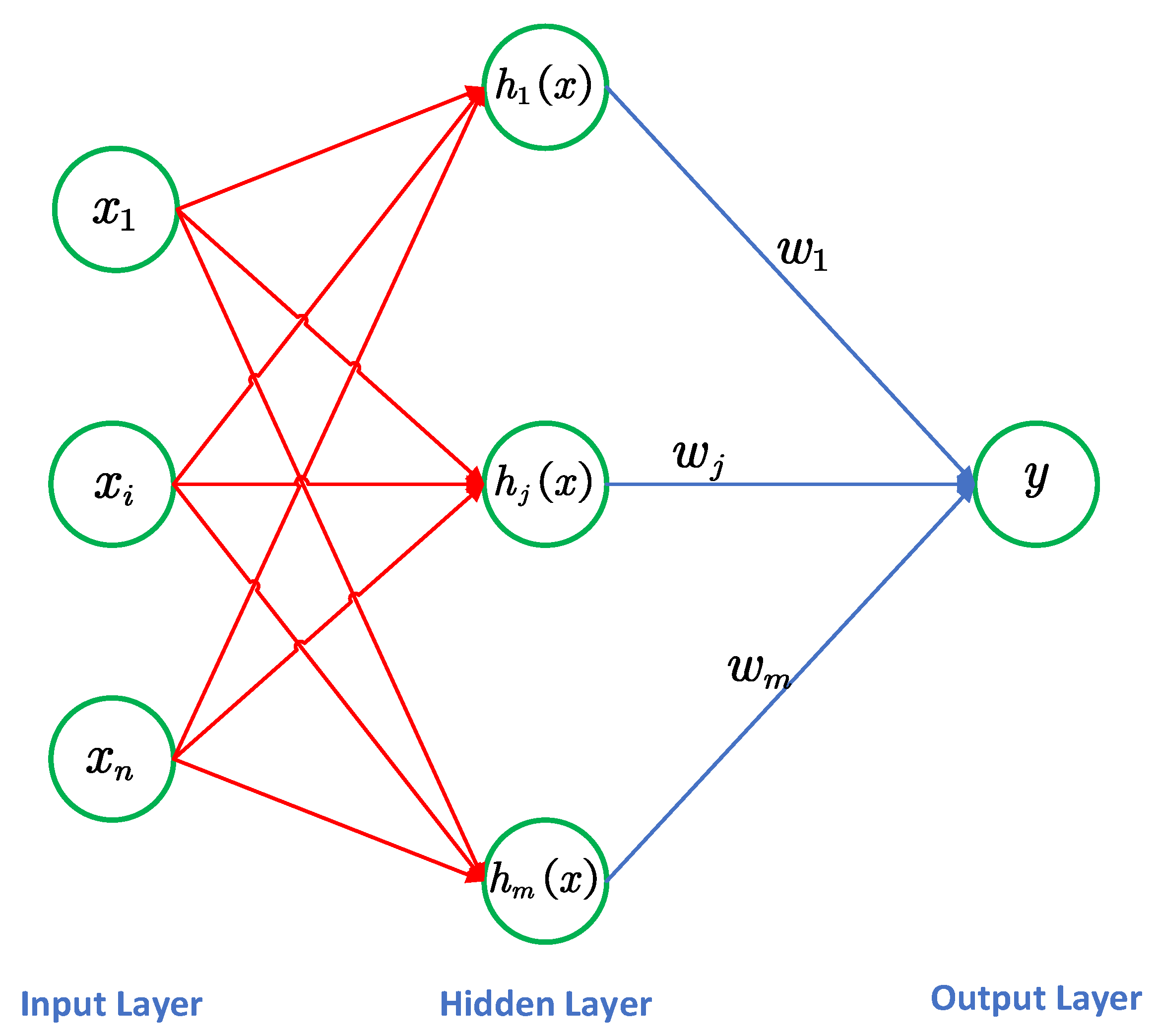
The RBF neural network is a three-layer feed-forward neural network in which the links from the input layer to the hidden layer are typically fixed and not trained. However, the links from the hidden layer to the output layer are trained. This is a simpler training process than that of standard neural network models [23].
The structure of the RBF neural network is shown in Figure 6.
In the RBF network structure, the input vector of the network is . The radial basis vector of the RBF network is , and the basis width vector of the hidden nodes of the network is . Then, the Gaussian basis function is
where is the center vector of the th hidden node of the network and is determined using the k-means training algorithm [24], and is the base width parameter of node .
The output of the RBF neural network is
where is the weight vector of the network and is determined via least squares approximation learning.
4.2. Improved Bootstrap Data Expansion Method Based on RBF Neural Network
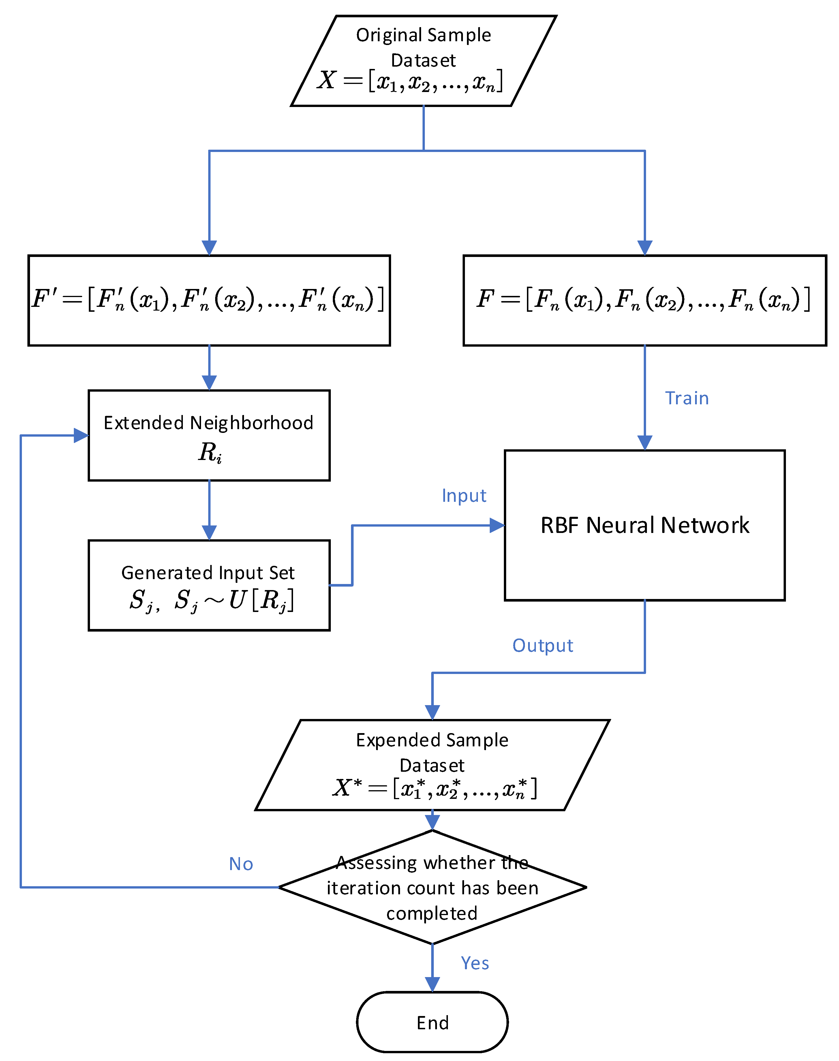
The methodology of the bootstrap data expansion method based on the RBF neural network is depicted in Figure 7.
First, the empirical distribution function expressed in Equation (5) is used to obtain the original sample dataset . The RBF neural network is trained based on the original sample dataset and the set of empirical distribution values . Notably, the effectiveness of this method has been demonstrated in [10]. Setting , the modified empirical distribution function in Equation (6) is then used to generate a set of empirical distributions based on the original sample dataset . As the RBF neural network produces more reliable outputs for inputs which are close to the training samples [25], a neighborhood function is introduced based on the input set. The expanded sample dataset is then obtained using the input set based on . The specific implementation steps are as follows.
- The original samples are sorted in descending order to obtain the order statistic of the sample , where , …, . Substituting into Equation (5) yields the set of empirical distribution values of , .
- RBF neural network training: The RBF neural network is trained by considering as the input and as the output of the network . The Gaussian radial basis function is used in the network, as shown in Equation (8).
- The neighborhood function of the set of empirical distributions is introduced. The input set of the RBF neural network is then obtained, and is substituted into Equation (6) to obtain the set of -corrected empirical distribution values . Let , and the neighborhood function bewhere is the neighborhood parameter (). The input set of the RBF neural network is generated sequentially from the uniform distribution of each neighborhood , where .
- The input set is fed into the RBF neural network to obtain the expanded sample . The elements of are input into the RBF neural network sequentially. When the input is , the output isThe set consisting of the RBF neural network outputs is the augmented sample of .
- Steps (3) and (4) are repeated times to obtain the expanded sample of .
4.3. Assessment of Reliability Indicators
After obtaining the expanded sample based on the maximum likelihood estimation of the two parameters of the Weibull distribution, the likelihood function for the shape parameter and the scale parameter is calculated according to the PDF in Equation (1), as follows:
where and are the shape parameter estimate and scale parameter estimate for the first entries of the expanded sample, respectively.
Applying the logarithmic function to Equation (12) yields the log-likelihood function.
The partial derivatives of the parameters and in Equation (13) are equal to 0. This results in two systems of equations, as follows.
Solving this system of equations yields and . Then, the mean time between failures (MTBF) is
Substituting Equation (1) into Equation (15) yields
Using variable substitution and the properties of the Gamma function, this integral can be simplified. The Gamma function is defined as follows:
Ultimately, the MTBF is
To ensure the accuracy of interval estimation, the method of bias correction is employed to estimate the confidence intervals. The center point of the confidence interval is modified by calculating the deviation between the original and expanded samples.
The normal quantile corresponding to the position of the original sample in the cumulative distribution function of the expanded sample distribution, , is calculated as
where denotes the inverse function of the cumulative distribution function of the standard normal distribution, i.e.,
I denotes the indicator function; N denotes the number of expanded samples; denotes the parameter estimates of the original sample; and denotes the parameter estimates of the th expansion sample.
The values of the parameter distributions of the expanded samples may not only be biased but also asymmetric, meaning that the width of the confidence intervals may need to be skewed. The acceleration value is used to modify the shape of the confidence interval and ensure that it adequately covers the true parameter values. In this study, the jackknife resampling method [26] is used to estimate the value of , as follows:
where is the sample size of the original sample, is the parameter estimate of the jackknife sample after excluding the th observation, and is the average of the parameter estimates of all the jackknife samples, i.e.,
Using the bias correction and the acceleration value , the upper and lower corrected quartiles of the confidence interval and are calculated as
where is the level of significance and is assumed to be 0.05.
Then, the confidence interval is
5. Example Analysis
Retrieve the maintenance records for seven CNC machines (designated as K1, K2, …, K7) operating under similar conditions within a single factory, spanning three years, to acquire 61 instances of failure data for this specific model (Table 3).
Point and interval estimation of the shape and scale parameters are performed using the maximum likelihood estimation method, bootstrap method, RBF + bootstrap method, and modified RBF + bootstrap method.
- Using the maximum likelihood estimation to estimate the parameters of the Weibull distribution for the original data yields and , and the reliability function is as follows:Then, MTBF is
- The conventional bootstrap method is used to expand the original data, and sampling is performed 1000 times, resulting in the expanded samples , . The overall distribution of is shown in Figure 8a.
Solving Equation (14) yields , and the average estimate is the following:
The parameter distribution obtained by solving Equation (18) for is shown in Figure 8b.
A mean value of is obtained, and the 95% confidence interval of is (1099.51, 1130.47), using the bias correction method.
- 3.
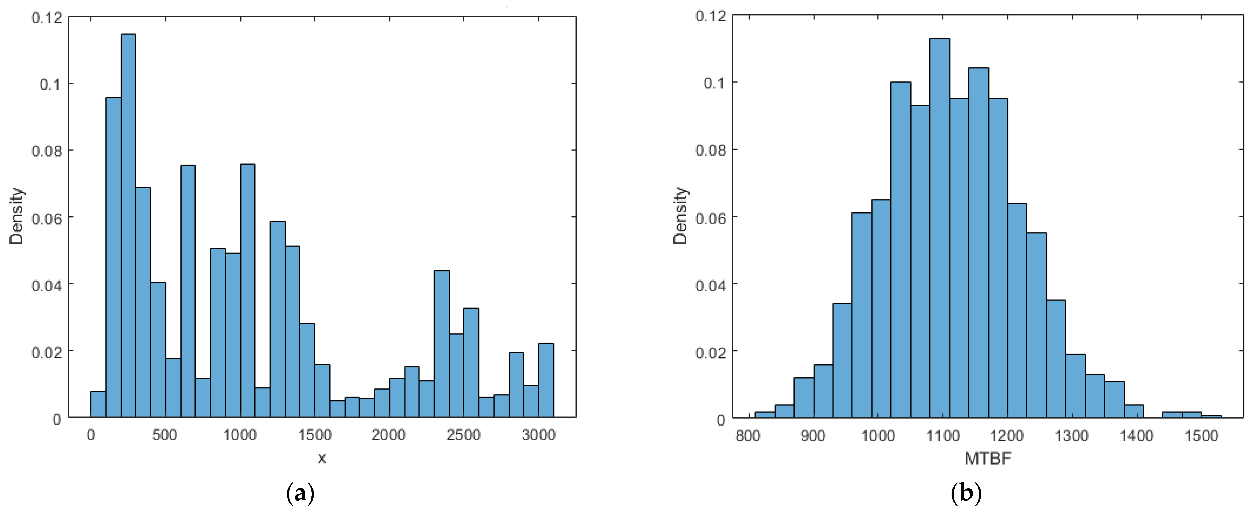
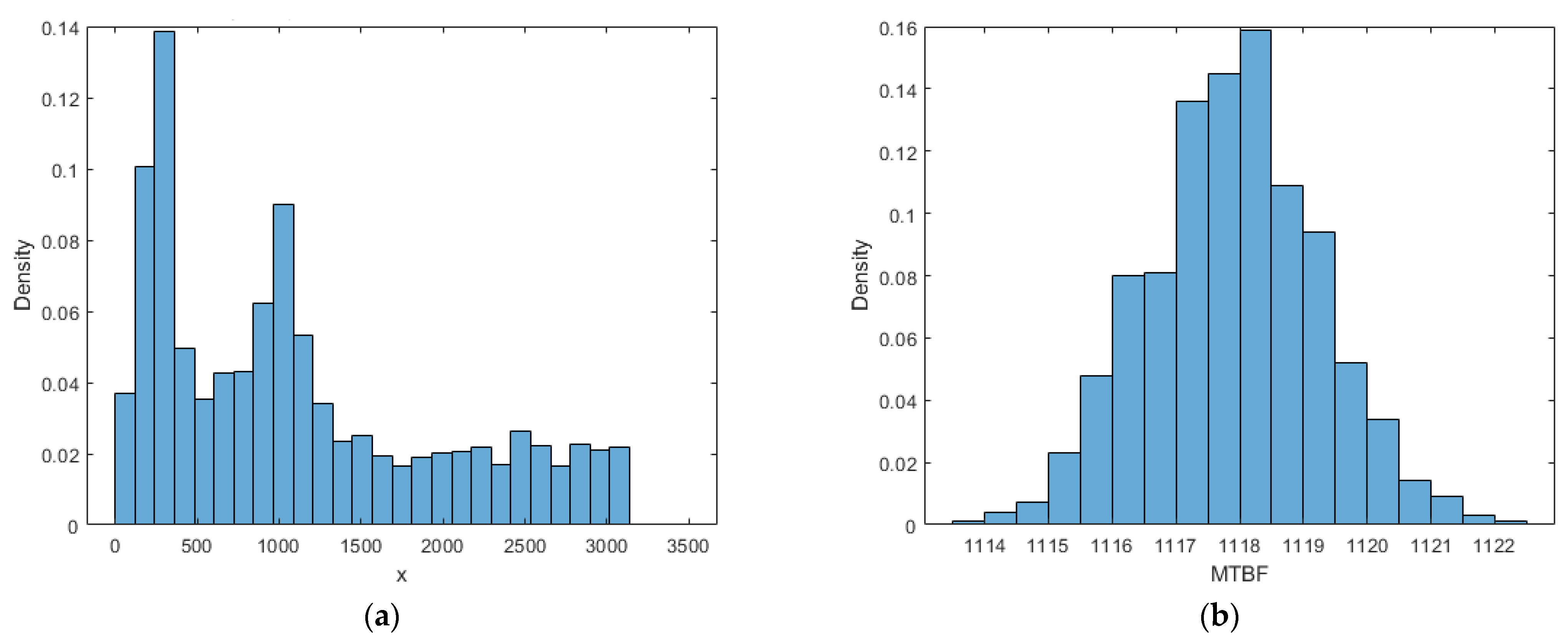
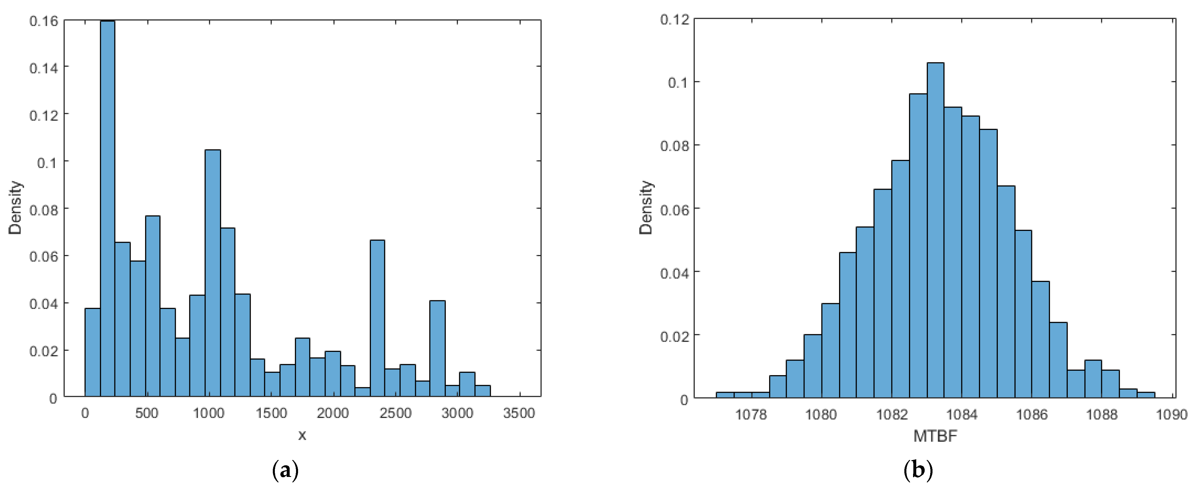
- The original data are expanded using the conventional bootstrap method and the improved bootstrap combined with the RBF neural network method. The “newrb” function in MATLAB (v2018b, MathWorks, Inc., Natick, MA, USA) is used to construct the RBF radial basis neural network. The network performance targets, expansion constants, and number of neurons, respectively, are set as . The calculation process is shown in Figure 7, and the results converge to yield the expanded samples of , , and . The average estimates of the Weibull parameters obtained using the conventional bootstrap method + RBF neural network are , with . The 95% confidence interval of is (1114.37, 1121.86), using the bias correction method. The average estimates of the Weibull parameters obtained using the improved bootstrap method + RBF neural network are , with . The 95% confidence interval of the obtained using the bias correction method is (1080.13, 1089.15). The overall distribution of is shown in Figure 9a, and the parameter distribution of is shown in Figure 9b. The overall distribution of is shown in Figure 10a, and the parameter distribution of is shown in Figure 10b.
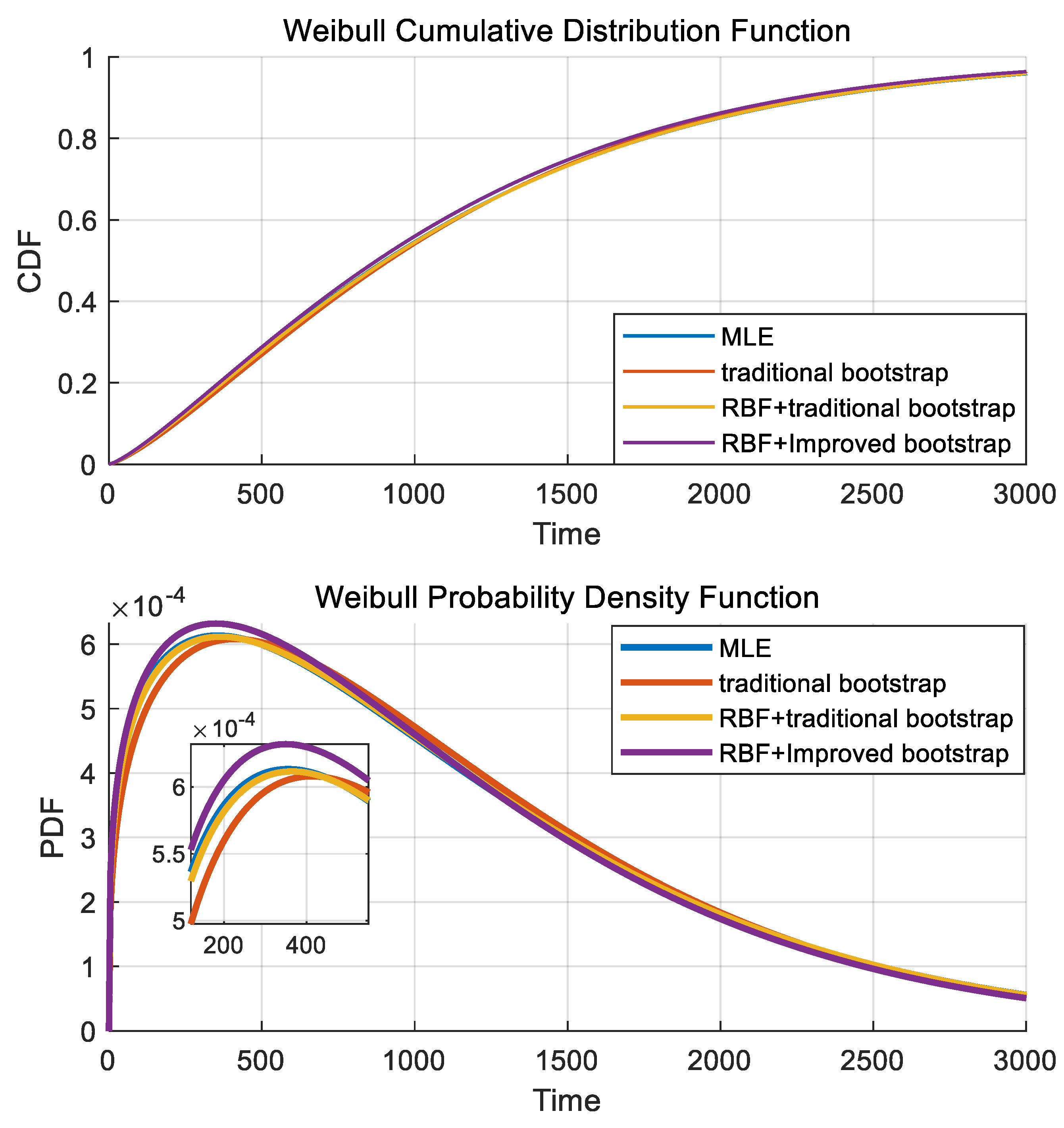
The cumulative distribution function (CDF) and probability density function (PDF) are obtained using Equations (1) and (2), as shown in Figure 11.
As illustrated in Figure 11, the probability density function (PDF) of the Weibull life distribution, obtained using the RBF plus the enhanced Bootstrap method, exhibits a peak value that is comparatively higher than those obtained through other methods. This observation can be interpreted as follows:
- A higher peak value indicates that the life data are more concentrated around a specific time period. This suggests that the majority of components or systems are likely to fail around this point in time, demonstrating a lower variability in life spans. In other words, the lifespans of most components are expected to be relatively similar, leading to reduced uncertainty in life expectancy predictions.
- Additionally, a higher peak value implies more accurate reliability predictions at this specific time point. Since failure events are more likely to occur near the peak, this facilitates more precise planning for maintenance, replacement cycles, and inventory management.
A comparison of the MTBF estimates obtained from the aforementioned methods with the manufacturer-rated MTBF = 1000 h and the corresponding errors are presented in Table 4.
As shown in Table 4, the estimated value of the MTBF obtained using the maximum likelihood estimation method is 1118.20 h, compared with the nominal value of 1000 h, resulting in a relative error of 11.82%. The relative error of the RBF + conventional bootstrap method is 11.83%, which is almost equal to that of the maximum likelihood estimation method, indicating that the expanded samples obtained using the RBF + conventional bootstrap method are overfitted and not sufficiently random for the bootstrap method. The analysis results presented in Figure 9a and Figure 10a reveal that correcting the tail of the empirical distribution function using an exponential distribution attenuates the proportion of large values and makes the distribution more dispersed, which is consistent with the actual life distribution of the equipment. In addition, the relative error for MTBF is reduced to 8.34% from 11.50%, indicating that the proposed data expansion method improves the conventional bootstrap method.
In this study, the confidence interval estimates for the different methods are obtained by combining bias correction methods. As shown in Table 4, the bootstrap method combined with the RBF neural network significantly reduces the length of the confidence intervals and improves the accuracy of the estimates. This demonstrates the effectiveness of combining RBF neural networks with the bootstrap method.
6. Conclusions
The estimation of equipment MTBF is crucial for reliability assessment and analysis. However, when the number of samples is limited, relying on traditional parameter estimation methods simulations is inadequate. Moreover, conventional parameter estimation methods such as maximum likelihood estimation typically fail to estimate the confidence intervals of the parameters.
This paper proposes the use of the bootstrap method for data expansion and reliability assessment. An exponential distribution is utilized to fit right-tailed data and modify the empirical distribution function. The simulation results indicate that the range of the expanded samples generated via the modified bootstrap method increases. The randomness of the expanded samples also increases, and the accuracy of interval estimation improves. In addition, a novel data expansion method is proposed by combining the modified bootstrap method with the RBF neural network. The bias correction method is then used to estimate confidence intervals for the expanded data and improve the estimation accuracy. Through our analysis of the results, this paper proposes that the method of tail data correction using an exponential function effectively enhances the original failure data by moderately incorporating additional information on the product’s reliability characteristics, based on its failure properties. This approach optimizes the raw data. Furthermore, employing the radial basis function (RBF) neural network essentially achieves a better fit of the failure data, thereby improving the accuracy of parameter estimation.
Finally, the proposed method is employed for the reliability assessment of a CNC machine tool. The shape and scale parameters of the corresponding Weibull distribution are estimated to determine the MTBF of the equipment. Simulation experiments show that the proposed method offers a greater improvement in the accuracy of point estimation and interval estimation than the original bootstrap and conventional parameter estimation methods. Therefore, this method has excellent applicability in engineering practice. Despite our research’s contributions, our work is not without limitations. The collection of CNC failure data presents significant challenges, notably due to the scarcity of available data. We compiled data from seven machines operating under ostensibly similar conditions, operating on the assumption that these conditions were identical. However, in reality, variances in operating conditions do exist. Addressing how to effectively integrate data across varying conditions represents a key area for our future investigations.
Author Contributions
Conceptualization, H.L. and H.W.; methodology, S.S.; software, H.W.; validation, H.L. and H.W.; formal analysis, H.W.; investigation, S.S.; resources, S.S.; data curation, H.W.; writing—original draft preparation, H.W.; writing—review and editing, H.L. and S.S. All authors have read and agreed to the published version of the manuscript.
Funding
This research received no external funding.
Institutional Review Board Statement
Not applicable.
Informed Consent Statement
Not applicable.
Data Availability Statement
The data presented in this study are available upon request from the corresponding author. The data are not publicly available due to privacy.
Acknowledgments
We extend our deepest appreciation to Zhang Zhihua for his invaluable guidance, unwavering support, and mentorship throughout this research.
Conflicts of Interest
The authors declare no conflicts of interest.
References
- Wilson, A.G.; Fronczyk, K.M. Bayesian reliability: Combining information. Qual. Eng. 2017, 29, 119–129. [Google Scholar] [CrossRef]
- Wang, L.; Pan, R.; Wang, X.; Fan, W.; Xuan, J. A Bayesian reliability evaluation method with different types of data from multiple sources. Reliab. Eng. Syst. Saf. 2017, 167, 128–135. [Google Scholar] [CrossRef]
- BahooToroody, A.; Abaei, M.M.; Banda, O.V.; Montewka, J.; Kujala, P. On reliability assessment of ship machinery system in different autonomy degree; A Bayesian-based approach. Ocean Eng. 2022, 254, 111252. [Google Scholar] [CrossRef]
- Efron, B. Bootstrap methods: Another look at the jackknife. In Breakthroughs in Statistics: Methodology and Distribution; Kotz, S., Johnson, N.L., Eds.; Springer: New York, NY, USA, 1992; pp. 569–593. [Google Scholar]
- Picheny, V.; Kim, N.H.; Haftka, R.T. Application of bootstrap method in conservative estimation of reliability with limited samples. Struct. Multidisc. Optim. 2010, 41, 205–217. [Google Scholar] [CrossRef]
- Amalnerkar, E.; Lee, T.H.; Lim, W. Reliability analysis using bootstrap information criterion for small sample size response functions. Struct. Multidisc. Optim. 2020, 62, 2901–2913. [Google Scholar] [CrossRef]
- Zhang, M.; Liu, X.; Wang, Y.; Wang, X. Parameter distribution characteristics of material fatigue life using improved bootstrap method. Int. J. Damage Mech. 2019, 28, 772–793. [Google Scholar] [CrossRef]
- Sun, H.; Hu, W.; Liu, H. Improvement of bayes bootstrap method based on interpolation method. Stat. Decis. 2017, 9, 74–77. [Google Scholar] [CrossRef]
- Zhao, Y.; Yang, L. Lifetime evaluation model of small sample based on Bootstrap theory. J. Beijing Univ. Aeronaut. Astronaut. 2022, 48, 106–112. [Google Scholar] [CrossRef]
- Tang, S.; Liu, G.; Li, X. A Bootstrap data expansion method based on RBF neural network and its application on IRSS reliability evaluation. China Meas. Test 2022, 48, 22–26. [Google Scholar]
- Zhang, C.W. Weibull parameter estimation and reliability analysis with zero-failure data from high-quality products. Reliab. Eng. Syst. Saf. 2021, 207, 107321. [Google Scholar] [CrossRef]
- Thanh Thach, T.; Briš, R. An additive Chen-Weibull distribution and its applications in reliability modeling. Qual. Reliab. Eng. Int. 2021, 37, 352–373. [Google Scholar] [CrossRef]
- Piña Monarrez, M.R.; Barraza-Contreras, J.M.; Villa-Señor, R.C. Vibration fatigue life reliability cable trough assessment by using Weibull distribution. Appl. Sci. 2023, 13, 4403. [Google Scholar] [CrossRef]
- Almarashi, A.M.; Algarni, A.; Nassar, M. On estimation procedures of stress-strength reliability for Weibull distribution with application. PLoS ONE 2020, 15, e0237997. [Google Scholar] [CrossRef]
- Poletto, J.P. An alternative to the exponential and Weibull reliability models. IEEE Access 2022, 10, 118759–118778. [Google Scholar] [CrossRef]
- Bai, H. A New Resampling Method to Improve Quality Research with Small Samples. Doctoral Dissertation, University of Cincinnati, Cincinnati, OH, USA, 2007. [Google Scholar]
- Larsen, J.E.P.; Lund, O.; Nielsen, M. Improved method for predicting linear B-cell epitopes. Immunome Res. 2006, 2, 1–7. [Google Scholar] [CrossRef]
- Linton, O.; Song, K.; Whang, Y.-J. An improved bootstrap test of stochastic dominance. J. Econom. 2010, 154, 186–202. [Google Scholar] [CrossRef]
- Ali, S.; Ali, S.; Shah, I.; Siddiqui, G.F.; Saba, T.; Rehman, A. Reliability analysis for electronic devices using generalized exponential distribution. IEEE Access 2020, 8, 108629–108644. [Google Scholar] [CrossRef]
- Collins, D.H.; Warr, R.L. Failure time distributions for complex equipment. Qual. Reliab. Eng. Int. 2019, 35, 146–154. [Google Scholar] [CrossRef]
- Chahkandi, M.; Ganjali, M. On some lifetime distributions with decreasing failure rate. Comput. Stat. Data Anal. 2009, 53, 4433–4440. [Google Scholar] [CrossRef]
- Xiao, G.; Li, T. Monte Carlo Method in System Reliability Analysis; Science Press: Beijing, China, 2003. [Google Scholar]
- Qian, J.; Chen, L.; Sun, J.-Q. Random vibration analysis of vibro-impact systems: RBF neural network method. Int. J. Non-Linear Mech. 2023, 148, 104261. [Google Scholar] [CrossRef]
- Sing, J.; Basu, D.; Nasipuri, M.; Kundu, M. Improved k-means algorithm in the design of RBF neural networks. In Proceedings of the TENCON 2003. Conference on Convergent Technologies for Asia-Pacific Region, Bangalore, India, 15–17 October 2003; pp. 841–845. [Google Scholar]
- Nabney, I.T. Efficient training of RBF networks for classification. Int. J. Neural Syst. 2004, 14, 201–208. [Google Scholar] [CrossRef] [PubMed]
- Hansen, B.E.; Racine, J.S. Jackknife model averaging. J. Econ. 2012, 167, 38–46. [Google Scholar] [CrossRef]
Figure 1.
Weibull distribution probability density function (PDF).

Figure 2.
Schematic of the bootstrap method.

Figure 3.
Distribution of original sample values.

Figure 4.
Distribution of sample values for expansion. (a) Conventional bootstrap; (b) improved bootstrap.
Figure 4.
Distribution of sample values for expansion. (a) Conventional bootstrap; (b) improved bootstrap.

Figure 5.
Parameter distribution of expanded samples. (a) Conventional bootstrap; (b) improved bootstrap.
Figure 5.
Parameter distribution of expanded samples. (a) Conventional bootstrap; (b) improved bootstrap.

Figure 6.
Schematic of the RBF neural network.

Figure 7.
Flowchart of the RBF + bootstrap approach.

Figure 8.
Results of the conventional bootstrap approach. (a) Overall distribution; (b) parametric distribution.
Figure 8.
Results of the conventional bootstrap approach. (a) Overall distribution; (b) parametric distribution.

Figure 9.
Results of the RBF + conventional bootstrap method. (a) Overall distribution; (b) parametric distribution.
Figure 9.
Results of the RBF + conventional bootstrap method. (a) Overall distribution; (b) parametric distribution.

Figure 10.
Results of the RBF + improved bootstrap method. (a) Overall distribution; (b) parametric distribution.
Figure 10.
Results of the RBF + improved bootstrap method. (a) Overall distribution; (b) parametric distribution.

Figure 11.
Plots of the cumulative distribution function (CDF) and probability density function (PDF).
Figure 11.
Plots of the cumulative distribution function (CDF) and probability density function (PDF).


Table 1.
Generated sample dataset.
| 51.67 | 64.43 | 85.08 | 102.42 | 151.11 |
| 52.27 | 68.97 | 88.70 | 113.02 | 152.14 |
| 56.96 | 74.02 | 88.88 | 115.54 | 159.35 |
| 57.38 | 74.20 | 91.13 | 120.89 | 160.67 |
| 61.56 | 76.24 | 94.91 | 131.71 | 164.48 |
| 63.95 | 77.65 | 100.55 | 147.34 | 166.26 |
Table 2.
Parameter () estimation table.
| Parameter Point Estimate | Estimation of Confidence Intervals | ||||
|---|---|---|---|---|---|
| Expected Value | Estimated Value | Error | Estimated Value | Interval Length | |
| Conventional bootstrap | 100.4493 | 99.7526 | 0.6967 | [99.1357, 100.6059] | 1.4702 |
| Improved bootstrap | 101.1103 | 0.6610 | [100.8831, 101.3135] | 0.4304 | |
Table 3.
Equipment failure data.
| Number | Time between Failures (h) | |||||
|---|---|---|---|---|---|---|
| K1 | 63.5 | 215.5 | 302 | 639.5 | 945.5 | 1264.25 |
| 2332.5 | 2591.5 | 2894 | ||||
| K2 | 178 | 318.08 | 374.5 | 645.5 | 1240.42 | 1246.58 |
| 1337 | 1419.5 | 2154 | ||||
| K3 | 215.3 | 230.17 | 837.33 | 838.67 | 1017.27 | 1486 |
| 2491.17 | 2842.33 | |||||
| K4 | 537.25 | 862.38 | 953.67 | 1027.67 | 1045.5 | 1274 |
| 1584 | 2449.25 | 3062.08 | ||||
| K5 | 194 | 271.5 | 399 | 913 | 1040 | 1873.5 |
| 2304.5 | 3062.5 | |||||
| K6 | 141.5 | 239.5 | 241.83 | 397.67 | 454.5 | 1382.5 |
| 2027.5 | 2312 | 2591.83 | ||||
| K7 | 153.5 | 184 | 186 | 409 | 639 | 655.5 |
| 686 | 1037 | 1375 | ||||
Table 4.
Comparison of reliability assessment results based on MTBF obtained using the different methods.
Table 4.
Comparison of reliability assessment results based on MTBF obtained using the different methods.
| Point Estimates (h) | Rated Value (h) | Absolute Error (h) | Relative Error (%) | Confidence Interval | Interval Length | |
|---|---|---|---|---|---|---|
| Maximum likelihood method | 1118.20 | 1000 | 118.20 | 11.82 | \ | \ |
| Bootstrap | 1114.97 | 114.97 | 11.50 | (1099.51, 1130.47) | 30.96 | |
| RBF + conventional bootstrap | 1118.32 | 118.32 | 11.83 | (1114.37, 1121.86) | 7.49 | |
| RBF +improved bootstrap | 1083.41 | 83.41 | 8.34 | (1080.13, 1089.15) | 9.02 |
Disclaimer/Publisher’s Note: The statements, opinions and data contained in all publications are solely those of the individual author(s) and contributor(s) and not of MDPI and/or the editor(s). MDPI and/or the editor(s) disclaim responsibility for any injury to people or property resulting from any ideas, methods, instructions or products referred to in the content. |
© 2024 by the authors. Licensee MDPI, Basel, Switzerland. This article is an open access article distributed under the terms and conditions of the Creative Commons Attribution (CC BY) license (https://creativecommons.org/licenses/by/4.0/).
Share and Cite
MDPI and ACS Style
Wang, H.; Liu, H.; Shao, S. Improved Bootstrap Method Based on RBF Neural Network for Reliability Assessment. Appl. Sci. 2024, 14, 2901. https://doi.org/10.3390/app14072901
AMA Style
Wang H, Liu H, Shao S. Improved Bootstrap Method Based on RBF Neural Network for Reliability Assessment. Applied Sciences. 2024; 14(7):2901. https://doi.org/10.3390/app14072901
Chicago/Turabian StyleWang, Houxiang, Haitao Liu, and Songshi Shao. 2024. "Improved Bootstrap Method Based on RBF Neural Network for Reliability Assessment" Applied Sciences 14, no. 7: 2901. https://doi.org/10.3390/app14072901
Note that from the first issue of 2016, this journal uses article numbers instead of page numbers. See further details here.